Chapter 16 Annotation

We developed and manually tested with few SNPs a method to match transcriptomic data from Tysklind et al., in prep with our genomic data. We found expected proportion of SNPs type, with a lot of putatively hitchhiker SNPs in functional SNPs. Finally, ca 2000 SNPs were matching between the two datasets.

population structure of individuals. Then, we quickly looked at th spatial and environmental distribution of the different gene pools and individual mismatch (before association genomic analyses).

• method data preparation and methodology to match transcriptomic data from Tysklind et al., in prep with our genomic data
• results SNP classification, corresponding SNPs and genes, and common SNPs between datasets.

16.1 Method

We focused on scaffolds from the hybrid genomic reference which contained a filtered SNP from the final dataset (7551 over 82792). We focused on transcripts longer than 500 bp and with at least one ORF (137 656 over 257 140). We then, used transcripts alignment on scaffolds to align back SNPs on transcripts, (beware the indexing position depend on the format vcf start with 1 while psl with 0). We proceeded as follow (not a common procedure but a home-made code to be double-checked):

1. SNP on scaffolds with no transcript match were classified as “purely neutral”
2. SNP on scaffolds matching a transcript were positioned on the global alignment
3. SNP out the alignment area were classified as “putatively hitchhiking”
4. SNP within the alignment area were further positionned among the different alignment blocks (cf blat functionning)
5. SNP out of alignment blocks (intron) were classified as “putatively hitchhiking”
6. SNP in one alignment blocks were classified as “functional”

scf <- read_tsv(file.path(path, "..", "variantCalling", "paracou",
                   "symcapture.all.biallelic.snp.filtered.nonmissing.paracou.bim"),
         col_names = c("scf", "snp", "posM", "pos", "A1", "A2")) %>% 
  dplyr::select(scf) %>% 
  unique() %>% 
  unlist()
reference <- readDNAStringSet(file.path(path, "..", "reference",  "reference.fasta"))
writeXStringSet(reference[scf],
                file.path(path, "scaffolds.fasta"))
orf <- src_sqlite(file.path("..", "..", "..", "data", "Symphonia_Genomic", "Niklas_transcripts",
                     "Trinotate", "symphonia.trinity500.trinotate.sqlite")) %>% 
  tbl("ORF") %>% 
  dplyr::select(transcript_id) %>% 
  dplyr::rename(trsc = transcript_id) %>% 
  collect() %>% 
  unique()
trsc.tbl <- src_sqlite(file.path("..", "..", "..", "data", "Symphonia_Genomic", "Niklas_transcripts",
                     "Trinotate", "symphonia.trinity500.trinotate.sqlite")) %>% 
  tbl("Transcript") %>% 
  dplyr::select(transcript_id, sequence) %>% 
  dplyr::rename(trsc = transcript_id) %>% 
  collect() %>% 
  filter(trsc %in% orf$trsc)
rm(orf)
trsc <- DNAStringSet(trsc.tbl$sequence)
names(trsc) <- trsc.tbl$trsc  
writeXStringSet(trsc, file.path(path, "transcripts.fasta"))
# blat scaffolds.fasta transcipts.fasta alignment.psl

16.2 Results

We obtained as planified a third of neutral snps (33%) against two thirds of non-neutral snps for which the majority was out of transcripts and may behave as hitchhikers (Fig. 16.1). Nevertheless, few functional snps matched several transcripts and/or genes due to transcripts isoforms, genes superposition and possibl multimatching errors (Fig. 16.2). For the moment we wont further annotate functional SNPs with ORFs and SNPs on transcript alignment, or gene ontology and synonymy. We will only finish annotation for selected SNPs in further analyses. Finally, we compared obtained SNP in genomics in this analysis with transcriptomic SNPs identified by Tysklind et al., in prep (Fig. 16.3)) and validated 2 098 common SNPs.

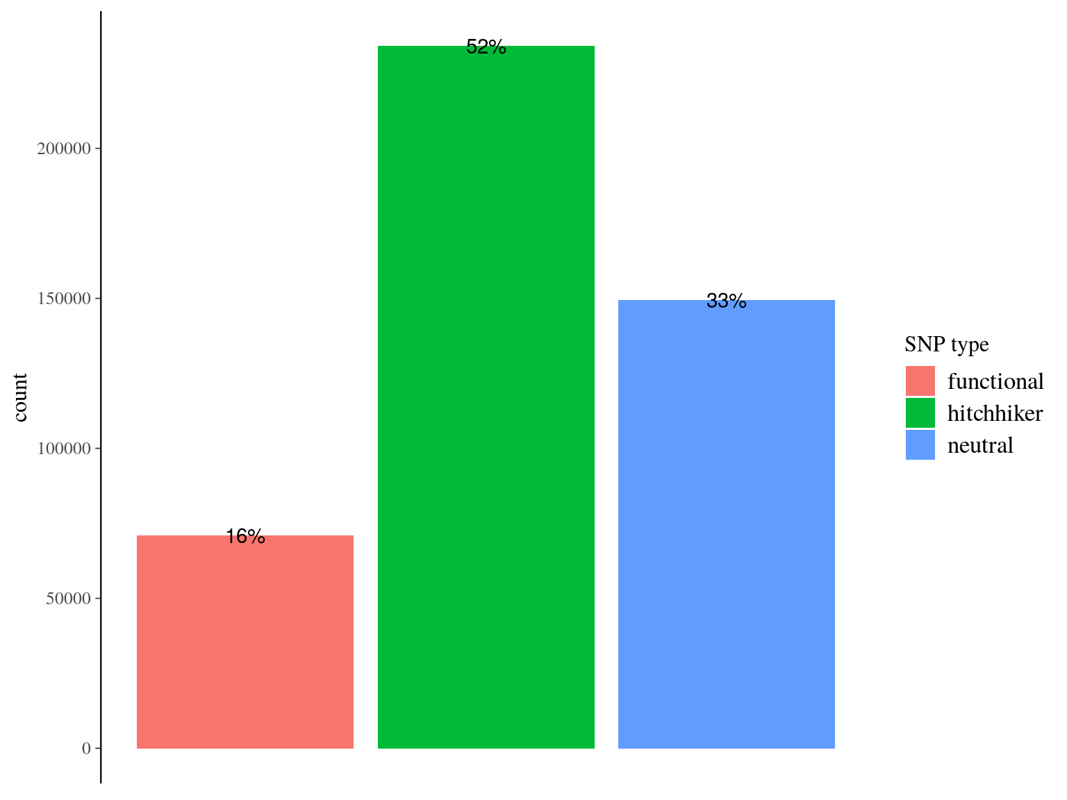
Figure 16.1: Filtered snps by type. SNP have been classified between (i) “purely neutral”, on scaffolds matching no transcript, (ii) “hitchhiker” on a scaffolds matching a trasncript but no within the transcript itself, and (iii) functional, when positioned within the matching transcript.

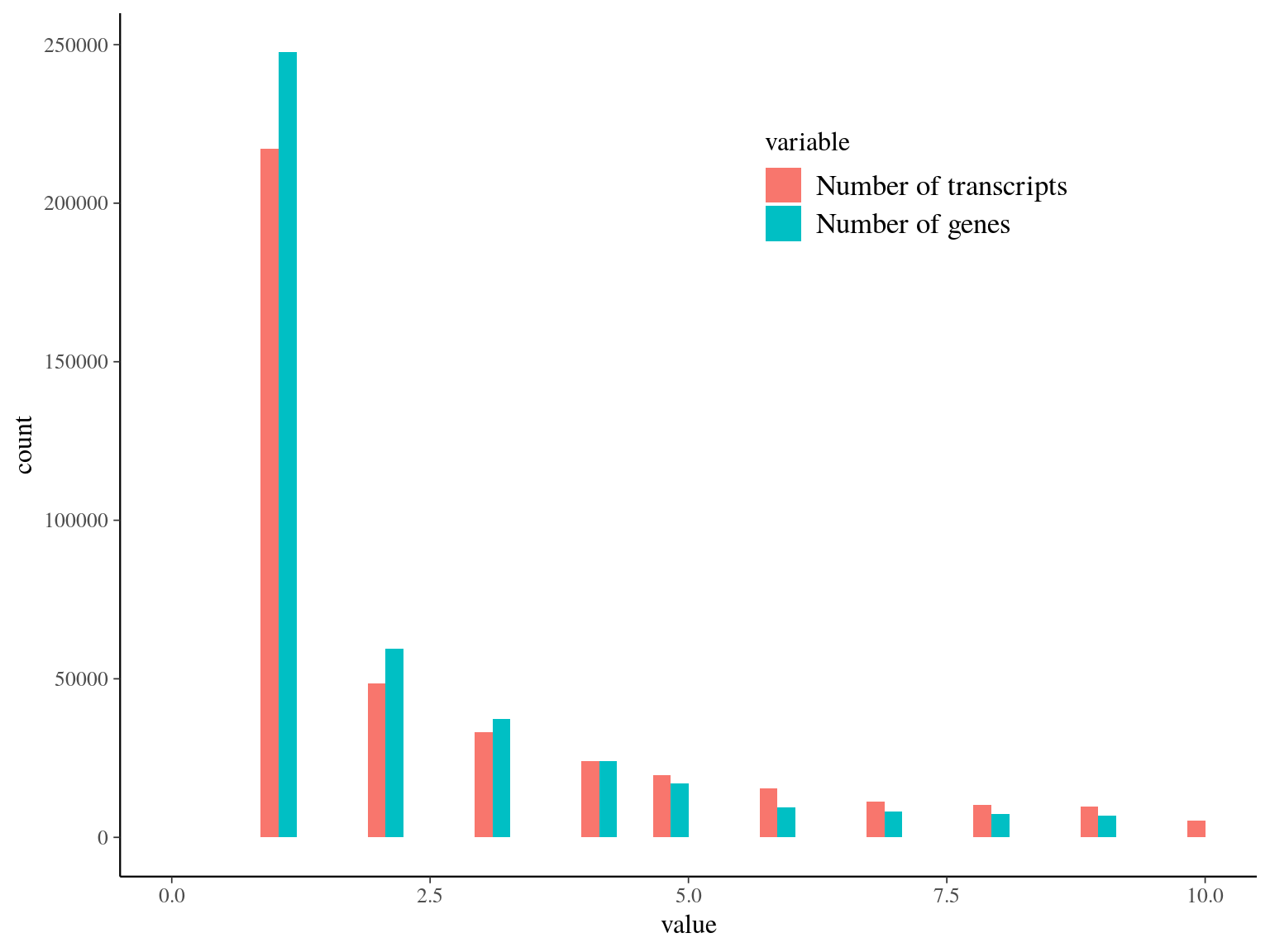
Figure 16.2: Transcripts and genes statistics per snp. Few snps have multiple transcripts, corresponding to different isoforms and/or multiple genes corresponding to orf superposition or multimatch error.

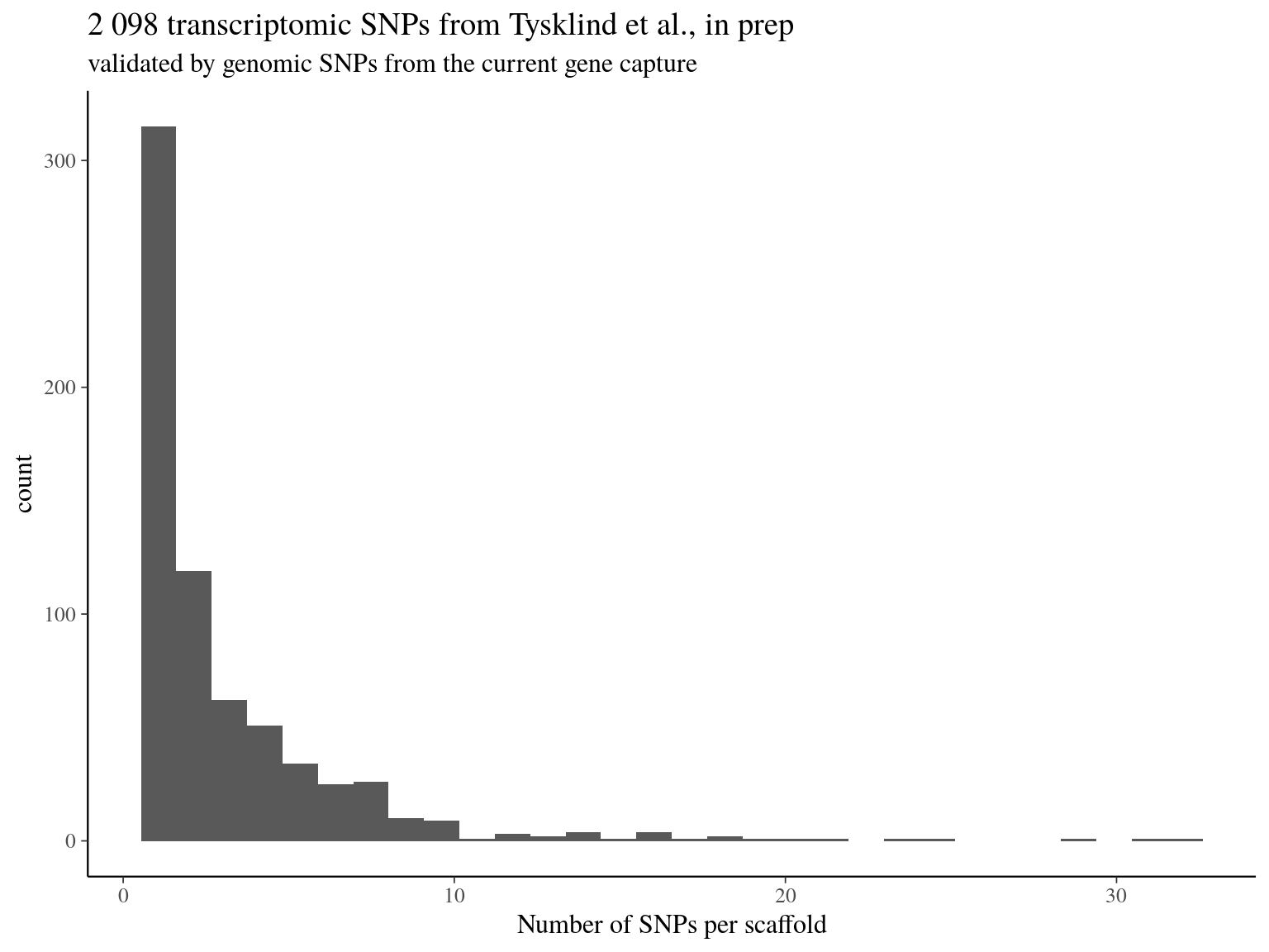
Figure 16.3: transcriptomic SNPs from Tysklind et al., in prep matching validated by genomic SNPs from the current gene capture.

cut -f2,9 snps.annotation > snps.type
grep neutral snps.type | cut -f1 > snps.neutral
grep hitchhiker snps.type | cut -f1 > snps.hitchhiker
grep functional snps.type | cut -f1 > snps.functional

16.3 Synonymy

snps <- read_tsv(file.path(path, "snpsFunc.annotation")) %>% 
  left_join(read_tsv(file.path(path, "snps.annotation")))
trsc <- src_sqlite(file.path("..", "..", "..", "data", "Symphonia_Genomic", "Niklas_transcripts",
                             "Trinotate", "symphonia.trinity500.trinotate.sqlite")) %>% 
  tbl("Transcript") %>% 
  filter(transcript_id %in% local(snps$trsc)) %>% 
  dplyr::rename(trsc = transcript_id) %>% 
  dplyr::select(trsc, sequence) %>% collect()
t <- snps %>% 
  dplyr::select(snp, trsc, posTrsc, A1, A2) %>% 
  reshape2::melt(id.vars = c("snp", "trsc", "posTrsc"), 
                 variable.name = "Allele", value.name = "base") %>% 
  arrange(snp) %>% 
  left_join(trsc) %>% 
  mutate(ref = stringr::str_sub(sequence, posTrsc, posTrsc)) %>%
  group_by(snp) %>% 
  filter(any(base %in% ref))
t %>% 
  filter(base != ref) %>% 
  ungroup() %>% 
  dplyr::select(trsc, posTrsc, base) %>% 
  write_tsv(path = file.path(path, "SNPsOnTrsc.tsv"), col_names = F)

mkdir TransDecoder
cp transcripts.fasta TransDecoder/
cd TransDecoder/
TransDecoder.LongOrfs -t transcripts.fasta
makeblastdb \
  -in /bank/ebi/uniprot/current/fasta/uniprot_sprot.fasta \
  -dbtype prot -input_type fasta -out uniprot/uniprot_sprot.fa -hash_index
blastp -query transcripts.fasta.transdecoder_dir/longest_orfs.pep \
  -db uniprot/uniprot_sprot.fa \
  -max_target_seqs 1 -outfmt 6 -evalue 1e-5 -num_threads 4 > blastp.outfmt6
hmmscan --cpu 4 --domtblout pfam.domtblout \
    Pfam/Pfam-A.hmm \
    transcripts.fasta.transdecoder_dir/longest_orfs.pep
TransDecoder.Predict -t transcripts.fasta \
    --retain_pfam_hits pfam.domtblout --retain_blastp_hits blastp.outfmt6
~/Tools/gffread/gffread longest_orfs.gff3 -T -o longest_orfs.gtf
perl ~/Tools/SNPdat_package_v1.0.5/SNPdat_v1.0.5.pl \
  -i SNPsOnTrsc.tsv \
  -g longest_orfs.gtf \
  -f transcripts.fasta \
  -s synonymy.summary \
  -o synonymy.output

snps <- read_tsv(file.path(path, "snpsFunc.annotation")) %>% 
  left_join(read_tsv(file.path(path, "snps.annotation")))
synonymy <- read_tsv(file.path(path, "synonymy.output"), col_names = T)
ggplot(synonymy, aes(synonymous)) + 
  geom_bar() +
  ggtitle(paste0(round(178908/475272*100), "% of non synonymous SNPs in genic SNPs"))
snps %>% 
  mutate(TRSC = toupper(trsc)) %>% 
  left_join(dplyr::rename(synonymy, TRSC = "Chromosome Number", posTrsc = "SNP Position")) %>% 
  dplyr::select(-TRSC) %>% 
  group_by(snp) %>% 
  summarise(synonymous = as.numeric(any(synonymous == "Y", na.rm = T))) %>% 
  mutate(synonymous = recode(synonymous, "1" = "synonymous", "0" = "anonymous")) %>% 
  write_tsv(path = file.path(path, "snpSynonymy.annotation"), col_names = F)
# grep synonymous snpSynonymy.annotation | cut -f1 > snp.synonymous
# grep anonymous snpSynonymy.annotation | cut -f1 > snp.anonymous