Chapter 17 Population history

We will … :

Phylogeny drift-based phylogeny with treemix for neutral and functional SNPs
Population diversity metrics ( $π$ , $F_{s t}$ and Tajima’s $D$ ) for neutral and functional SNPs
Site Frequency Structure per population and between populations for neutral and functional SNPs

17.1 Drift-based Phylogeny - `treemix`

We used representative individuals from S. sp1, S. globulifera type Paracou, and S. globulifera type Régina, in association with South American (La Selva, Baro Colorado Island, and Itubera) and African (Madagascar, Benin, Cameroun, Sao Tome, Congo, Benin, Liberia, Gana and Ivory Coast) Symphonia and Pentadesma to explore population phylogeny with treemix (Fig. 17.1). We built phylogeny for the neutral, hitchhiker, and functional SNPs. All datasets suggested 1 migration event to better represent the phylogeny than none. Topology was the same between dataset, functional SNP just show less drift than others.

module load bioinfo/plink-v1.90b5.3
cp symcapture.all.biallelic.snp.filtered.nonmissing.treemix.bim symcapture.all.biallelic.snp.filtered.nonmissing.treemix.bim0
awk '{print $1"\t"$1"_snp"$4"\t"$3"\t"$4"\t"$5"\t"$6}' symcapture.all.biallelic.snp.filtered.nonmissing.treemix.bim0 > symcapture.all.biallelic.snp.filtered.nonmissing.treemix.bim
rm symcapture.all.biallelic.snp.filtered.nonmissing.treemix.bim0
plink --bfile all/symcapture.all.biallelic.snp.filtered.nonmissing.treemix \
  --allow-extra-chr \
  --freq --missing --within symcapture.all.biallelic.snp.filtered.nonmissing.treemix.pop \
  --out all/symcapture.all.biallelic.snp.filtered.nonmissing.treemix
plink --bfile all/symcapture.all.biallelic.snp.filtered.nonmissing.treemix \
  --extract snps.functional \
  --allow-extra-chr \
  --freq --missing --within symcapture.all.biallelic.snp.filtered.nonmissing.treemix.pop \
  --out functional/symcapture.all.biallelic.snp.filtered.nonmissing.treemix
plink --bfile all/symcapture.all.biallelic.snp.filtered.nonmissing.treemix \
  --extract snps.hitchhiker \
  --allow-extra-chr \
  --freq --missing --within symcapture.all.biallelic.snp.filtered.nonmissing.treemix.pop \
  --out hitchhiker/symcapture.all.biallelic.snp.filtered.nonmissing.treemix
plink --bfile all/symcapture.all.biallelic.snp.filtered.nonmissing.treemix \
  --extract snps.neutral \
  --allow-extra-chr \
  --freq --missing --within symcapture.all.biallelic.snp.filtered.nonmissing.treemix.pop \
  --out neutral/symcapture.all.biallelic.snp.filtered.nonmissing.treemix
gzip */symcapture.all.biallelic.snp.filtered.nonmissing.treemix.frq.strat
python plink2treemix.py all/symcapture.all.biallelic.snp.filtered.nonmissing.treemix.frq.strat.gz treemix.all.frq.gz 
python plink2treemix.py neutral/symcapture.all.biallelic.snp.filtered.nonmissing.treemix.frq.strat.gz treemix.neutral.frq.gz 
python plink2treemix.py functional/symcapture.all.biallelic.snp.filtered.nonmissing.treemix.frq.strat.gz treemix.functional.frq.gz 
python plink2treemix.py hitchhiker/symcapture.all.biallelic.snp.filtered.nonmissing.treemix.frq.strat.gz treemix.hitchhiker.frq.gz 
cp *.frq.gz ../../populationGenomics/treemix
cd ../../populationGenomics/treemix
module load bioinfo/treemix-1.13
treemix -i treemix.frq.gz -root Madagascar -o out
for m in $(seq 10) ; do treemix -i treemix.frq.gz -root Madagascar -m $m -g out.vertices.gz out.edges.gz -o out$m ; done
grep Exiting *.llik > migration.llik

Drift-based phylogeny of *Symphonia* and *Pentadesma* populations with `treemix` [@Pickrell2012]. Subfigure **A** present the log-likelihood of the phylogeny topology depending on the number of allowed migration events per SNP type, suggesting 1 migration event to better represent the phylogeny topology than none. Others subfigures represent the phylogeny for anonymous (**B**), genic (**C**) and putatively-hitchhiker (**D**) SNPs. The red arrow represents the most likely migration event. Population are named by their localities, including *Symphonia* species only or *Symphonia* and *Pentadesma* species in Africa. At the exception of the three Paracou populations: *S. sp1*, *S. globulifera type Paracou* and *S. globulifera type Regina* respectivelly named Ssp1, SgParacou and SgRegina.

Figure 17.1: Drift-based phylogeny of Symphonia and Pentadesma populations with treemix (Pickrell & Pritchard 2012). Subfigure A present the log-likelihood of the phylogeny topology depending on the number of allowed migration events per SNP type, suggesting 1 migration event to better represent the phylogeny topology than none. Others subfigures represent the phylogeny for anonymous (B), genic (C) and putatively-hitchhiker (D) SNPs. The red arrow represents the most likely migration event. Population are named by their localities, including Symphonia species only or Symphonia and Pentadesma species in Africa. At the exception of the three Paracou populations: S. sp1, S. globulifera type Paracou and S. globulifera type Regina respectivelly named Ssp1, SgParacou and SgRegina.

17.2 Population diversity

After defining populations based on our 3 gene pools (S. sp.1, S. globulifera type Paracou, and S. globulifera type Regina) with more than 90% of mebership to the gene pool in admixture, we used vcftools to compute nucleotide diversity $π$ , population differentiation $F_{s t}$ , and Tajima’s $D$ per SNP type (functional, hitchhiker or neutral).

cp symcapture.all.biallelic.snp.filtered.nonmissing.paracou3pop.bim symcapture.all.biallelic.snp.filtered.nonmissing.paracou3pop.bim0
awk '{print $1"\t"$1"_snp"$4"\t"$3"\t"$4"\t"$5"\t"$6}' symcapture.all.biallelic.snp.filtered.nonmissing.paracou3pop.bim0 > symcapture.all.biallelic.snp.filtered.nonmissing.paracou3pop.bim
rm symcapture.all.biallelic.snp.filtered.nonmissing.paracou3pop.bim0
module load bioinfo/plink-v1.90b5.3
types=(neutral hitchhiker functional)
for type in "${types[@]}" ; 
  do 
  plink \
    --bfile symcapture.all.biallelic.snp.filtered.nonmissing.paracou3pop \
    --allow-extra-chr \
    --extract snps.$type \
    --recode vcf-iid \
    -out paracou3pop.$type &
done
grep sp1 paracou3pop.popmap | cut -f1 > sp1.list
grep globuliferaTypeParacou paracou3pop.popmap | cut -f1 > globuliferaTypeParacou.list
grep globuliferaTypeRegina paracou3pop.popmap | cut -f1 > globuliferaTypeRegina.list

17.2.1 $π$

Nucleotide diversity $π$ per site had a mean of 0.05140 across populations and was significantly different between populations (ANOVA, p<2e-16) with S. globulifera type Regina being more diverse (Fig. 17.2). No significant differences existed between SNP types.

types=(neutral hitchhiker functional)
pops=(sp1 globuliferaTypeParacou globuliferaTypeRegina) 
for type in "${types[@]}" ; 
  do 
  for pop in "${pops[@]}" ; 
    do 
    vcftools --vcf paracou3pop.$type.vcf --keep $pop.list --site-pi --out $type.$pop &
  done
done
types=(synonymous anonymous)
pops=(sp1 globuliferaTypeParacou globuliferaTypeRegina) 
for type in "${types[@]}" ; 
  do 
  for pop in "${pops[@]}" ; 
    do 
    vcftools --vcf paracou3pop.$type.vcf --keep $pop.list --window-pi 100 --out $type.$pop &
  done
done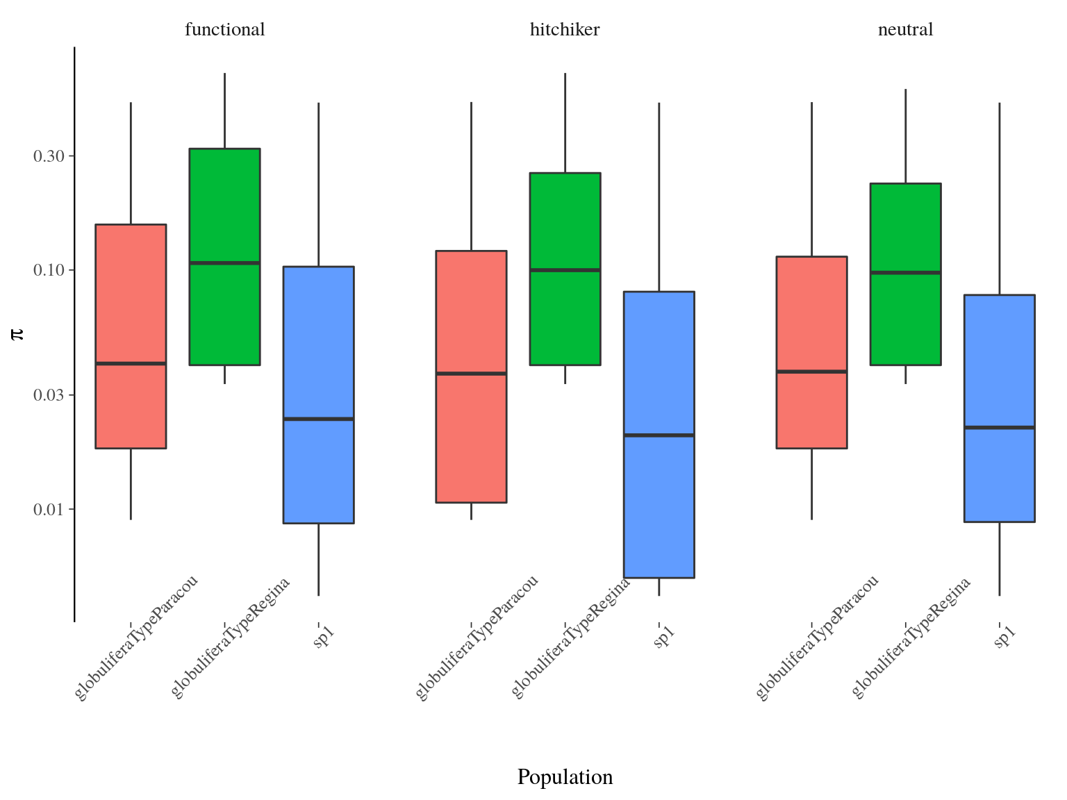

$Populations $\pi$ distribution estimated by `vcftools` per site.$

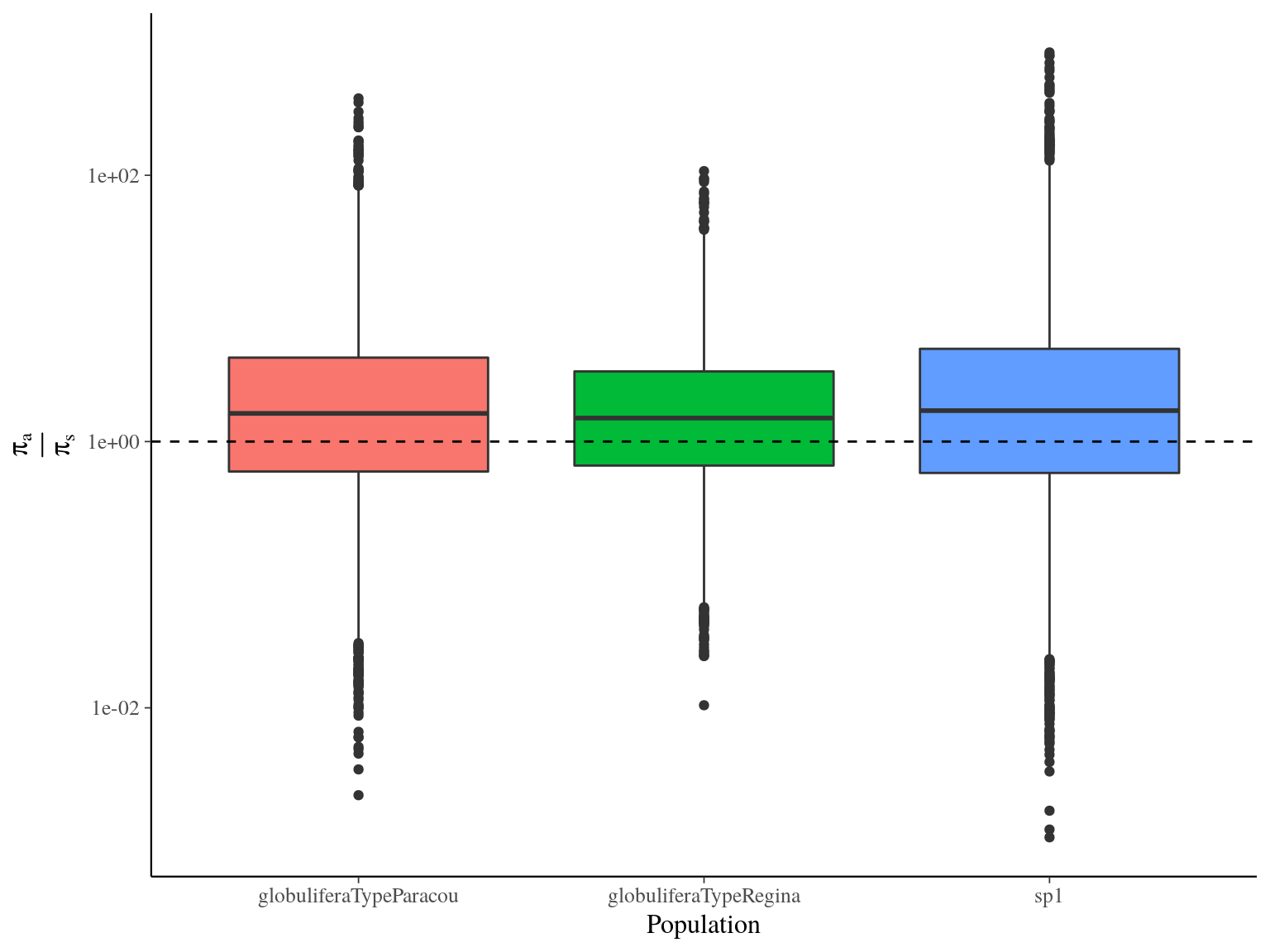
Figure 17.2: Populations $π$ distribution estimated by vcftools per site.

$Populations $\frac{\pi_a}{\pi_s}$ distribution estimated by `vcftools` on a 100 bp window.$

Figure 17.3: Populations $\frac{π_{a}}{π_{s}}$ distribution estimated by vcftools on a 100 bp window.

17.2.2 $F_{s t}$

$F_{s t}$ between population was globally low with a mean value of 0.15, still S. globulifera type Regina was more differentiated to the two toher gene pools (Fig. 17.4) for every SNP type. Nevertheless, functional SNP were significantly less differentiated than hitchhikers and neutral SNPs.

types=(neutral hitchhiker functional)
pop1=(sp1 sp1 globuliferaTypeParacou) 
pop2=(globuliferaTypeParacou globuliferaTypeRegina globuliferaTypeRegina) 
for type in "${types[@]}" ; 
  do 
  for i in $(seq 3) ; 
    do 
    vcftools --vcf paracou3pop.$type.vcf \
      --weir-fst-pop "${pop1[i-1]}".list \
      --weir-fst-pop "${pop2[i-1]}".list \
      --out $type."${pop1[i-1]}"_"${pop2[i-1]}" &
  done
done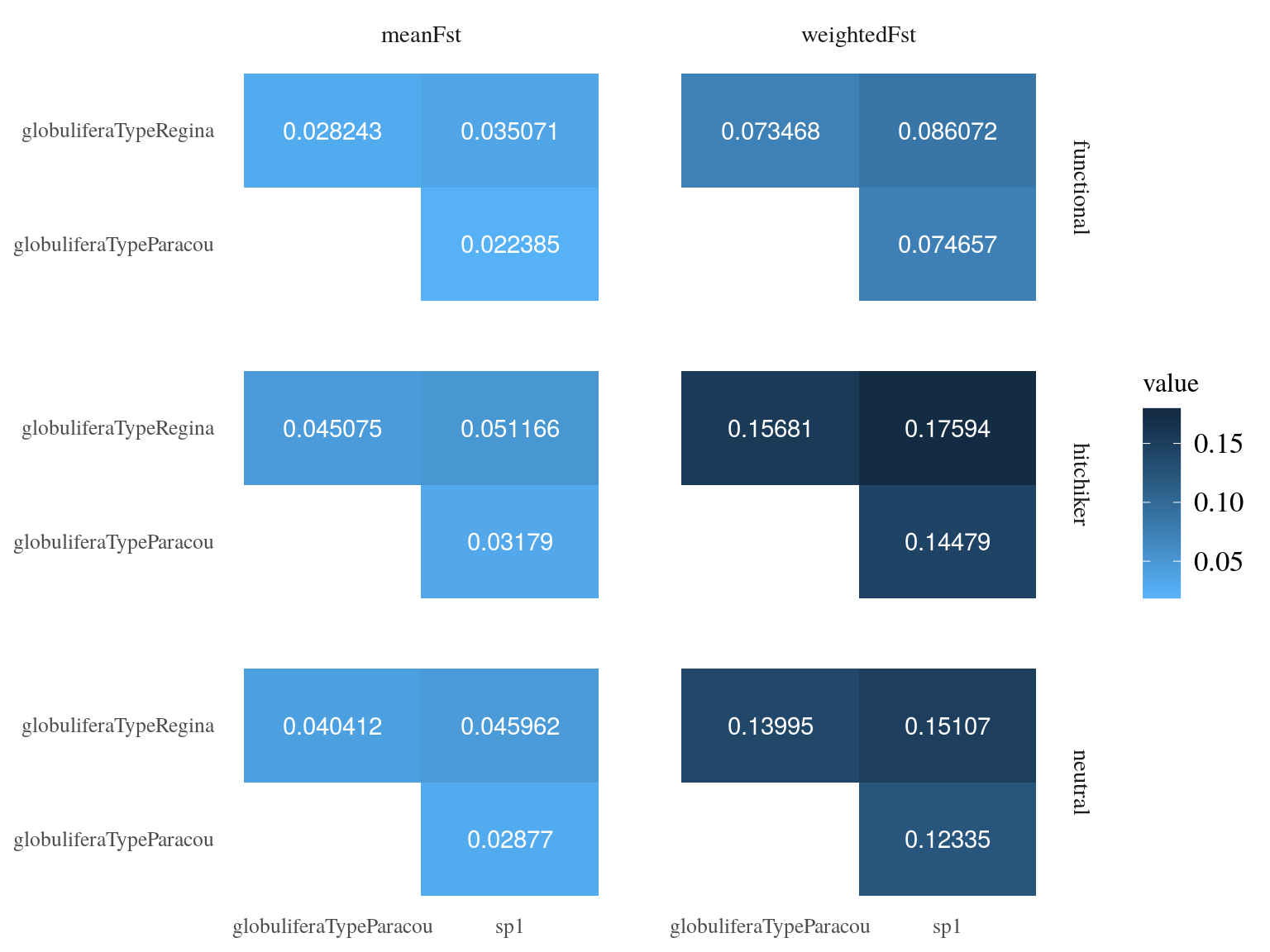

Figure 17.4: Between populations Fst estimated by vcftools.

17.2.3 Tajima’s $D$

Tajima’s $D$ between population was globally low and significantly negative with a mean value of -0.795 and was significantly different between populations (ANOVA, p<2e-16) with S. globulifera type Regina having a globally higher value (Fig. 17.5). We expect positive selection (or selective sweeps) to give us a negative Tajima’s $D$ in a population that doesn’t have any demographic changes going on (population expansion/contraction, migration, etc). On the other hand with balancing selection, alleles are kept at intermediate frequencies. This produces a positive Tajima’s $D$ because there will be more pairwise differences than segregating sites. Consequently, Tajima’s $D$ indicates here that are population are under selection with a stronger selection operating on S. globulifera type Paracou and S. sp1 than S. globulifera type Regina. No significant differences existed between SNP types.

types=(neutral hitchhiker functional)
pops=(sp1 globuliferaTypeParacou globuliferaTypeRegina) 
for type in "${types[@]}" ; 
  do 
  for pop in "${pops[@]}" ; 
    do 
    vcftools --vcf paracou3pop.$type.vcf --keep $pop.list --TajimaD 100 --out $type.$pop &
  done
done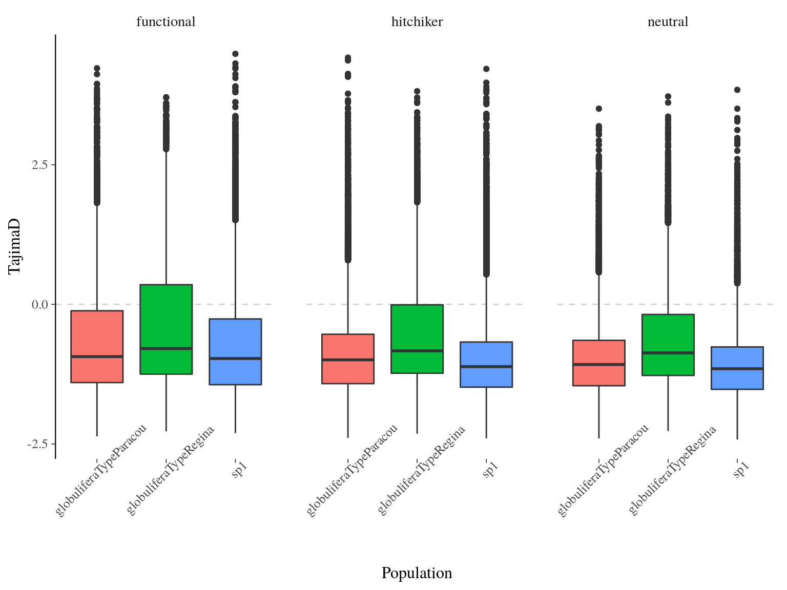

Figure 17.5: Populations Tajima’s D distribution estimated by vcftools on windows of 100 bp.

17.3 Site Frequency Structure

Berlin presentation

cp symcapture.all.biallelic.snp.filtered.nonmissing.paracouWeighted3pop.bim symcapture.all.biallelic.snp.filtered.nonmissing.paracouWeighted3pop.bim0
awk '{print $1"\t"$1"_snp"$4"\t"$3"\t"$4"\t"$5"\t"$6}' symcapture.all.biallelic.snp.filtered.nonmissing.paracouWeighted3pop.bim0 > symcapture.all.biallelic.snp.filtered.nonmissing.paracouWeighted3pop.bim
rm symcapture.all.biallelic.snp.filtered.nonmissing.paracouWeighted3pop.bim0
module load bioinfo/plink-v1.90b5.3
types=(neutral hitchhiker functional)
for type in "${types[@]}" ; 
  do 
  plink \
    --bfile symcapture.all.biallelic.snp.filtered.nonmissing.paracouWeighted3pop \
    --allow-extra-chr \
    --extract snps.$type \
    --recode vcf-iid \
    -out paracouWeighted3pop.$type &
done

source("https://raw.githubusercontent.com/shenglin-liu/vcf2sfs/master/vcf2sfs.r")
prefix <- file.path(path, "SFS", "paracouWeighted3pop")
pops <- c("sp1", "globuliferaTypeParacou", "globuliferaTypeRegina")
types <- c("neutral", "hitchhiker", "functional")
for(type in types)
  for(pop in pops){
    vcf2dadi(paste0(prefix, ".", type, ".vcf"), 
             paste0(prefix, ".popmap"), 
             paste0(prefix, ".", type, ".", pop, ".dadi"), 
             pop)
    dadi2fsc.1pop(paste0(prefix, ".", type, ".", pop, ".dadi"), 
                  paste0(prefix, ".", type, ".", pop, ".fastsim"),
                  pop, fold = T)
  }
popPairs <- combn(pops,2)
for(type in types)
  for(i in 1:ncol(popPairs)){
  vcf2dadi(paste0(prefix, ".", type, ".vcf"), 
           paste0(prefix, ".popmap"),
           paste0(prefix, ".", type, ".", popPairs[1,i], "_", popPairs[2,i], ".dadi"), 
           popPairs[,i])
  dadi2fsc.2pop(paste0(prefix, ".", type, ".", popPairs[1,i], "_", popPairs[2,i], ".dadi"), 
                paste0(prefix, ".", type, ".", popPairs[1,i], "_", popPairs[2,i], ".fastsim"),
                popPairs[,i], fold = T)
}

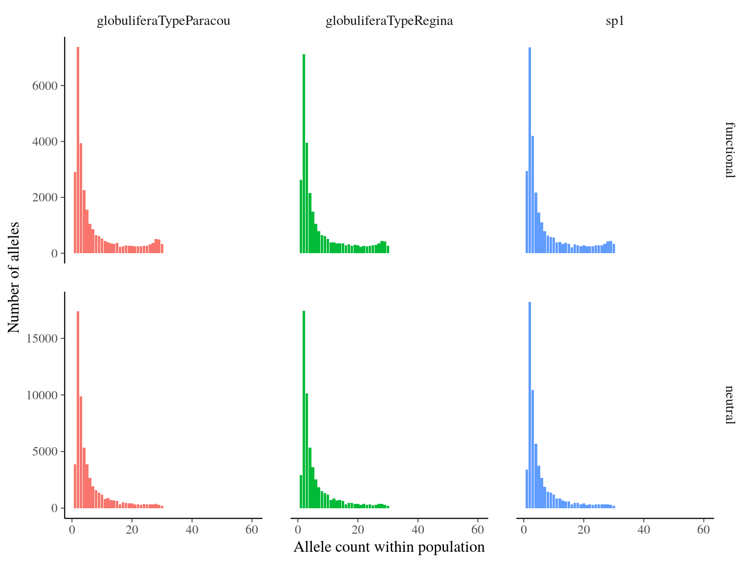
Figure 17.6: Number of alleles per allele count and population.

Figure 17.7: Number of alleles per allele count between population.

References

Pickrell, J.K. & Pritchard, J.K. (2012). Inference of Population Splits and Mixtures from Genome-Wide Allele Frequency Data. PLoS Genetics, 8.

Chapter 17 Population history

17.1 Drift-based Phylogeny - treemix