Chapter 19 Growth & Animal models
The aim of this document is to explore animal and growth model with generated data to validate their behavior and use it on Symphonia and Eschweilera real data. Let’s consider a set of \(P=3\) populations including each \(Fam=3\) families composed of \(I = 14\) individuals with arbitrar relationships (it’s only 126 individuals to do quick tests).
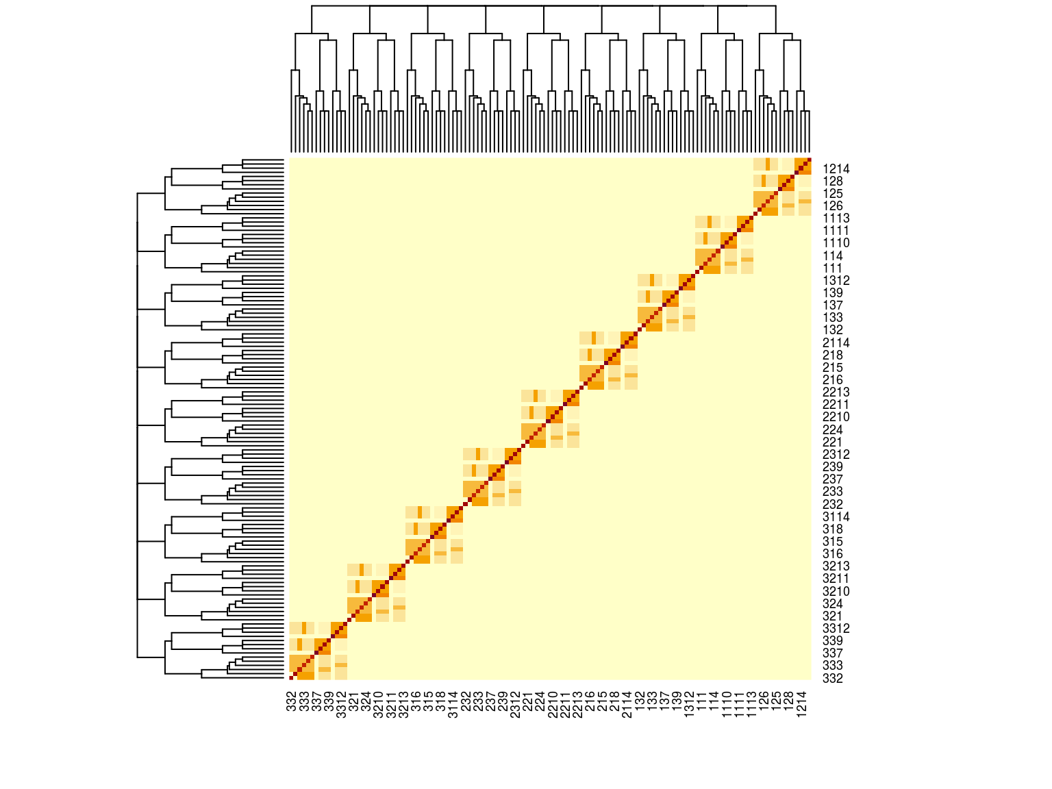
Figure 19.1: Kinship matrix
19.1 Animal
We used the following animal model with a lognormal distribution to estimate population and genotypic variance:
\[\begin{equation} y_{p,i} \sim \mathcal{logN}(log(\mu_p.a_{i}),\sigma_1) \\ a_{p,i} \sim \mathcal{MVlogN_N}(log(1),\sigma_2.K) \tag{19.1} \end{equation}\]
We fitted the equivalent model with following priors:
\[\begin{equation} y_{p,i} \sim \mathcal{logN}(log(\mu_p.\hat{a_{i}}), \sigma_1) \\ \hat{a_{i}} = e^{\sqrt{V_G}.A.\epsilon_i} \\ \epsilon_i \sim \mathcal{N}(0,1) \\ ~ \\ \mu_p \sim \mathcal{logN}(log(1),1) \\ \sigma_1 \sim \mathcal N_T(0,1) \\ ~ \\ V_Y = Var(log(y)) \\ V_P = Var(log(\mu_p)) \\ V_R=\sigma_1^2 \\ V_G = V_Y - V_P - V_R \\ \tag{19.2} \end{equation}\]
| Parameter | Estimate | Expected | Standard error | \(\hat R\) |
|---|---|---|---|---|
| mu[1] | 0.7473821 | 0.7357714 | 0.0535640 | 1.0054690 |
| mu[2] | 0.3992248 | 0.3633681 | 0.0308554 | 1.0010121 |
| mu[3] | 0.5209272 | 0.5420625 | 0.0469693 | 1.0023625 |
| Vp | 0.0702100 | 0.0841187 | 0.0151127 | 1.0011662 |
| Vg | 0.0770262 | 0.0837454 | 0.0223466 | 1.0014673 |
| Vr | 0.0399184 | 0.0400000 | 0.0145103 | 0.9997977 |
| lp__ | 78.5632162 | NA | 22.6506583 | 1.0019419 |
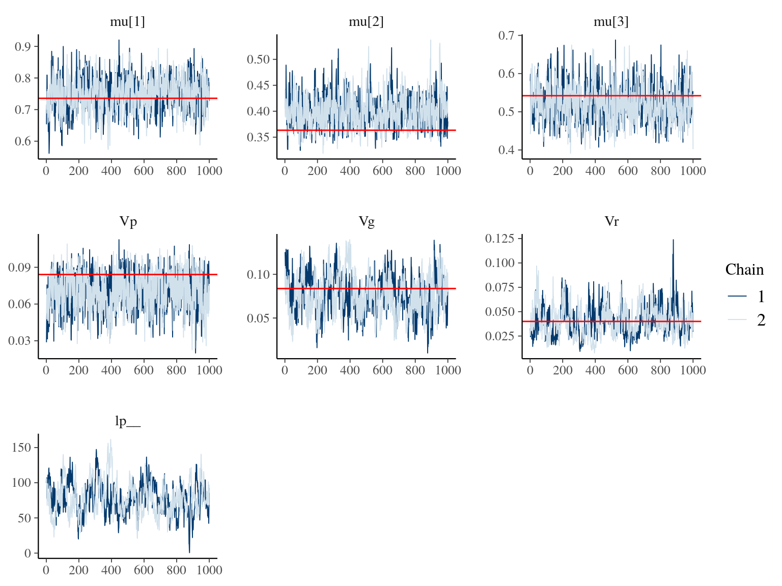
Figure 19.2: Parameters for Animal model traceplot and expected value in red.
19.2 Gmax
We used the following growth model with a lognormal distribution to estimate individual growth potential:
\[\begin{equation} DBH_{y=today,p,i} - DBH_{y=y0,p,i} \sim \\ \mathcal{logN} (log(\sum _{y=y_0} ^{y=today} \theta_{1,p,i}.exp(-\frac12.[\frac{log(\frac{DBH_{y,p,i}}{100.\theta_{2,p}})}{\theta_{3,p}}]^2)), \sigma_1) \\ \theta_{1,p,i} \sim \mathcal {logN}(log(\theta_{1,p}), \sigma_2) \\ \theta_{2,p} \sim \mathcal {logN}(log(\theta_2),\sigma_3) \\ \theta_{3,p} \sim \mathcal {logN}(log(\theta_3),\sigma_4) \tag{19.3} \end{equation}\]
We fitted the equivalent model with following priors:
\[\begin{equation} DBH_{y=today,p,i} - DBH_{y=y0,p,i} \sim \\ \mathcal{logN} (log(\sum _{y=y_0} ^{y=today} \hat{\theta_{1,p,i}}.exp(-\frac12.[\frac{log(\frac{DBH_{y,p,i}}{100.\hat{\theta_{2,p}}})}{\hat{\theta_{3,p}}}]^2)), \sigma_1) \\ \hat{\theta_{1,p,i}} = e^{log(\theta_{1,p}) + \sigma_2.\epsilon_{1,i}} \\ \hat{\theta_{2,p}} = e^{log(\theta_2) + \sigma_3.\epsilon_{2,p}} \\ \hat{\theta_{3,p}} = e^{log(\theta_3) + \sigma_4.\epsilon_{3,p}} \\ \epsilon_{1,i} \sim \mathcal{N}(0,1) \\ \epsilon_{2,p} \sim \mathcal{N}(0,1) \\ \epsilon_{3,p} \sim \mathcal{N}(0,1) \\ ~ \\ (\theta_{1,p}, \theta_2, \theta_3) \sim \mathcal{logN}^3(log(1),1) \\ (\sigma_1, \sigma_2, \sigma_3, \sigma_4) \sim \mathcal{N}^4_T(0,1) \\ ~ \\ V_P = Var(log(\mu_p)) \\ V_R=\sigma_2^2 \tag{19.4} \end{equation}\]
| Parameter | Estimate | Standard error | Expected | \(\hat R\) |
|---|---|---|---|---|
| thetap1[1] | 0.5300911 | 0.0976327 | 0.5300000 | 1.0084649 |
| thetap1[2] | 0.5872973 | 0.1001450 | 0.5400000 | 1.0145937 |
| thetap1[3] | 0.3946491 | 0.0508020 | 0.3600000 | 1.0073573 |
| theta2 | 0.2572377 | 0.1007272 | 0.2500000 | 1.0000859 |
| theta3 | 0.5907776 | 0.1029564 | 0.7000000 | 0.9991474 |
| Vp | 0.0458205 | 0.0326534 | 0.0376656 | 1.0177764 |
| Vr | 0.4342078 | 0.0897607 | 0.4489000 | 1.1038441 |
| lp__ | 102.6878571 | 95.9191313 | NA | 1.6993161 |
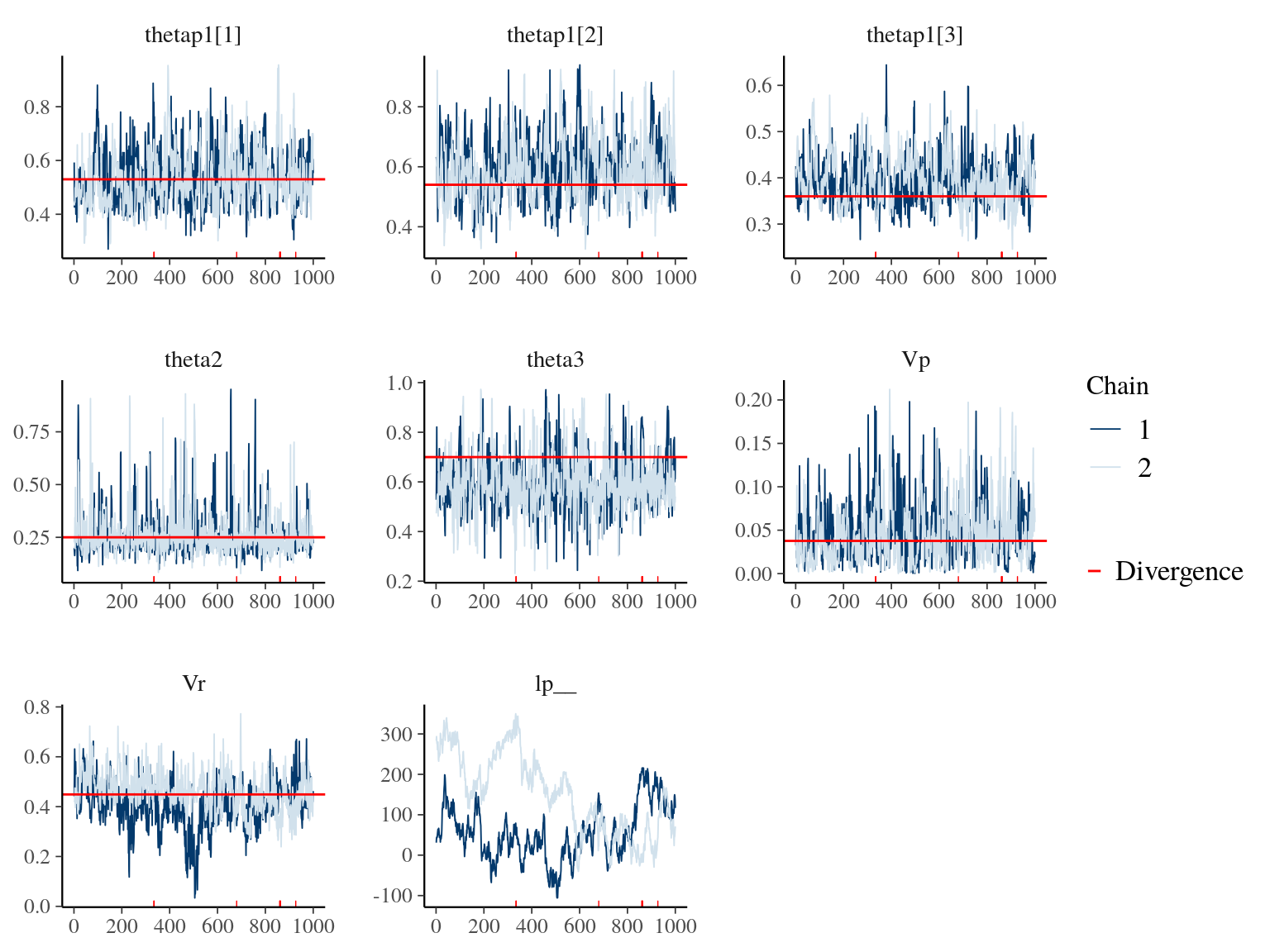
Figure 19.3: Parameters for Growth model traceplot and expected value in red.
19.3 Gmax & Animal
We used the following growth model with a lognormal distribution to estimate individual growth potential and associated genotypic variation:
\[\begin{equation} DBH_{y=today,p,i} - DBH_{y=y0,p,i} \sim \\ \mathcal{logN} (log(\sum _{y=y_0} ^{y=today} \theta_{1,p,i}.exp(-\frac12.[\frac{log(\frac{DBH_{y,p,i}}{100.\theta_{2,p}})}{\theta_{3,p}}]^2)), \sigma_1) \\ \theta_{1,p,i} \sim \mathcal {logN}(log(\theta_{1,p}.a_{1,i}), \sigma_2) \\ \theta_{2,p} \sim \mathcal {logN}(log(\theta_2),\sigma_3) \\ \theta_{3,p} \sim \mathcal {logN}(log(\theta_3),\sigma_4) \\ a_{1,i} \sim \mathcal{MVlogN}(log(1), \sigma_5.K) \tag{19.5} \end{equation}\]
We fitted the equivalent model with following priors:
\[\begin{equation} DBH_{y=today,p,i} - DBH_{y=y0,p,i} \sim \\ \mathcal{logN} (log(\sum _{y=y_0} ^{y=today} \hat{\theta_{1,p,i}}.exp(-\frac12.[\frac{log(\frac{DBH_{y,p,i}}{100.\hat{\theta_{2,p}}})}{\hat{\theta_{3,p}}}]^2)), \sigma_1) \\ \hat{\theta_{1,p,i}} = e^{log(\theta_{1,p}.\hat{a_{1,i}}) + \sigma_2.\epsilon_{1,i}} \\ \hat{\theta_{2,p}} = e^{log(\theta_2) + \sigma_3.\epsilon_{2,p}} \\ \hat{\theta_{3,p}} = e^{log(\theta_3) + \sigma_4.\epsilon_{3,p}} \\ \hat{a_{1,i}} = e^{\sigma_5.A.\epsilon_{4,i}} \\ \epsilon_{1,i} \sim \mathcal{N}(0,1) \\ \epsilon_{2,p} \sim \mathcal{N}(0,1) \\ \epsilon_{3,p} \sim \mathcal{N}(0,1) \\ \epsilon_{4,i} \sim \mathcal{N}(0,1) \\ ~ \\ (\theta_{1,p}, \theta_2, \theta_3) \sim \mathcal{logN}^3(log(1),1) \\ (\sigma_1, \sigma_2, \sigma_3, \sigma_4, \sigma_5) \sim \mathcal{N}^5_T(0,1) \\ ~ \\ V_P = Var(log(\mu_p)) \\ V_G=\sigma_5^2\\ V_R=\sigma_2^2 \tag{19.6} \end{equation}\]
| Parameter | Estimate | Standard error | Expected | \(\hat R\) |
|---|---|---|---|---|
| thetap1[1] | 0.8158910 | 0.1121729 | 0.5300000 | 1.0008119 |
| thetap1[2] | 0.4921939 | 0.0889950 | 0.5400000 | 1.0015447 |
| thetap1[3] | 0.3495413 | 0.0629704 | 0.3600000 | 1.0009558 |
| theta2 | 0.2756253 | 0.0764302 | 0.2500000 | 1.0004898 |
| theta3 | 0.7269206 | 0.1440250 | 0.7000000 | 0.9996955 |
| Vp | 0.1414014 | 0.0635966 | 0.0352066 | 1.0016146 |
| Vg | 0.0558953 | 0.0758363 | 0.1350074 | 1.0016744 |
| Vr | 0.5172295 | 0.1090083 | 0.4489000 | 1.0170006 |
| lp__ | 36.7247279 | 66.4530270 | NA | 1.1521719 |
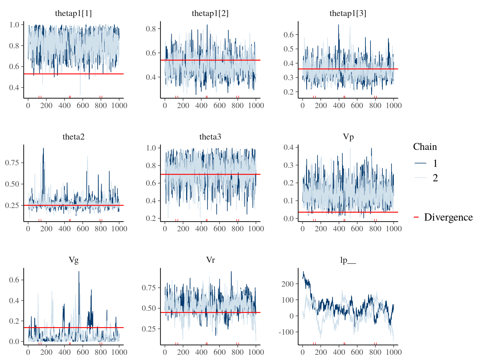
Figure 19.4: Parameters for Growth & Animal model traceplot and expected value in red.