Chapter 20 Environmental genomics
We explored and selected environmental descriptors to be used in environmental genomics. We then used the three methods to quantify and explore the link between variable environemental variation and individual SNP and kinship variation with:
- the modele Animal to explore genetic variance associated to the environemntal variable
- linear mixed models (LMM) used to identify major effect SNPs associated to the environemntal variable
20.1 Descriptors
The topographic wetness index (TWI) was selected among several abiotic descriptors as a proxy of water accumulation. Waterlogging and topography have been highlighted as crucial for forest dynamics (Ferry et al. 2010) and species habitat preference (Allié et al. 2015) at the Paracou study site. TWI was derived from a 1-m resolution digital elevation model using SAGA-GIS (Conrad et al. 2015) based on a LiDAR campaign done in 2015.
Biotic descriptors included the Neighborhood Crowding Index (NCI; Uriarte et al. 2004) and the Annual Crowding Rate, both integrated over time. The Neighborhood Crowding Index \(NCI_i\) from tree individual \(i\) was calculated with following formula:
\[\begin{equation} NCI_i = (\int_{t_0} ^{2015} \sum _{j~|~\delta_{i,j}<20m} ^{J_{i,t}} DBH_{j,t}^2 e^{-\frac14.\delta_{i,j}}.dt).\frac1{\Delta t} \tag{20.1} \end{equation}\]
with \(DBH_j\) the diameter from neighboring tree \(j\) and \(\delta_{i,j}\) its distance to individual tree \(i\). \(NCI_i\) is computed for all neighbors at a distance \(\delta_{i,j}\) inferior to maximum neighboring distance of 20 meters. The power of neighbors \(DBH\) effect was set to 2 to consider neighbors surface. The decrease of neighbors \(DBH\) effect with distance was set to 0.25 here to represent trees at 20 meters of the focal trees having 1% of the effect of the same tree at 0 meters. \(NCI\) represents biotic asymmetric competition through tree neighborhood over time. Both correlations and principal component analyses showed non colinear TWI and NCI that we selected for further analyses (Fig. ??).
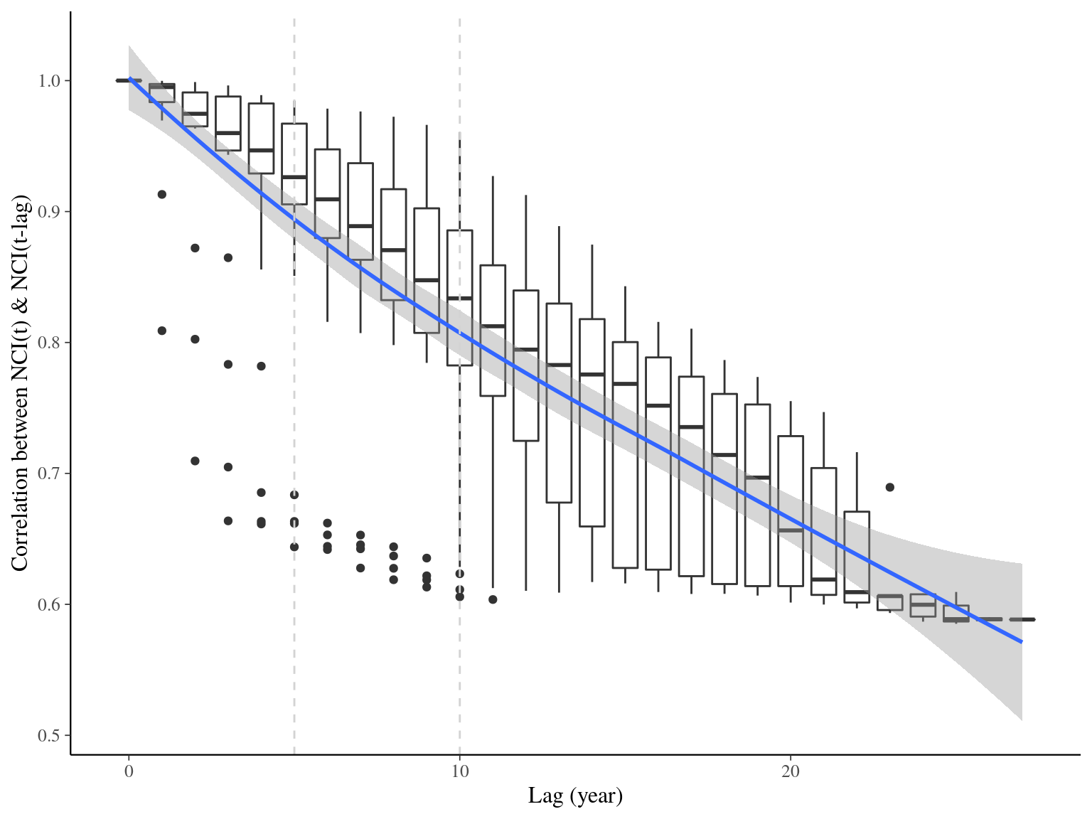
Figure 20.1: Temporal autocorrelation for NCI.
20.2 Genetic variance
We used between individual kinship and a lognormal Animal model (Wilson et al. 2010) to estimate genetic variance associated to individuals global phenotype leaving in a given environment (see environmental association analyses with genome wide assocaition study analyses in Rellstab et al. 2015). Animal model is calculated for the environemental values \(y\) of the \(N\) individuals with following formula:
\[\begin{equation} y_{p,i} \sim \mathcal{logN}(log(a_{p,i}),\sigma_1) \\ a_{p,i} \sim \mathcal{MVlogN_N}(log(\mu_p),\sigma_2.K) \tag{20.2} \end{equation}\]
where individual is defined as a normal law centered on the individual genetic additive effects \(a\) and associated individual remaining variance \(\sigma_R\). Additive genetic variance \(a\) follow a multivariate lognormal law centered on the population mean \(\mu_{Population}\) of covariance \(\sigma_G K\).
We fitted the equivalent model with following priors:
\[\begin{equation} y_{p,i} \sim \mathcal{logN}(log(\mu_p) + \hat{\sigma_2}.A.\epsilon_i, \sigma_1) \\ \epsilon_i \sim \mathcal{N}(0,1) \\ ~ \\ \mu_p \sim \mathcal{logN}(log(1),1) \\ \sigma_1 \sim \mathcal N_T(0,1) \\ \hat{\sigma_2} = \sqrt(V_G) ~ \\ V_Y = Var(log(y)) \\ V_P = Var(log(\mu_p)) \\ V_G = V_Y - V_P - V_R \\ V_R=\sigma_1^2 \tag{20.3} \end{equation}\]
The model converged (Fig. 20.2) well for TWI but had some known diffuclties (see previous chapter) for NCI due to a low residual variation (\(V_{R,NCI}=0.04\)). We had two constrated results with most of the explained variation mainly attributed to the genotype for NCI (85%) and the majority attributed to population for TWI (42%). Still population explained 12% of NCI and genotype 4% of TWI. Finally, remaining variattion was almost null (3%) for NCI whereas important for TWI (54%) (Tab. 20.1 and Fig. ?? and 20.4).
| Variable | Parameter | Population | Estimate | \(\sigma\) | \(\hat{R}\) |
|---|---|---|---|---|---|
| TWI | mu | S. globulifera Paracou | 1.0764330 | 0.0561835 | 1.0130283 |
| TWI | mu | S. globulifera Regina | 1.3021745 | 0.1147511 | 1.0133244 |
| TWI | mu | S. sp1 | 0.5698126 | 0.0208222 | 1.0025316 |
| TWI | Vp | 0.1110215 | 0.0129248 | 1.0041464 | |
| TWI | Vg | 0.0375413 | 0.0309989 | 1.0694287 | |
| TWI | Vr | 0.1707870 | 0.0294494 | 1.0643870 | |
| RE | mu | S. globulifera Paracou | 1.1533814 | 0.0377264 | 1.0021073 |
| RE | mu | S. globulifera Regina | 1.1090129 | 0.0681339 | 1.0004498 |
| RE | mu | S. sp1 | 1.9164534 | 0.0473329 | 1.0016365 |
| RE | Vp | 0.0634923 | 0.0061197 | 0.9999994 | |
| RE | Vg | 0.0142252 | 0.0121362 | 1.0198243 | |
| RE | Vr | 0.0861835 | 0.0121037 | 1.0170763 | |
| NCI | mu | S. globulifera Paracou | 0.7892597 | 0.0305778 | 0.9997771 |
| NCI | mu | S. globulifera Regina | 0.9466499 | 0.0643210 | 1.0003822 |
| NCI | mu | S. sp1 | 0.9427773 | 0.0290419 | 1.0012267 |
| NCI | Vp | 0.0074662 | 0.0033377 | 1.0004033 | |
| NCI | Vg | 0.0251105 | 0.0193455 | 1.0640539 | |
| NCI | Vr | 0.0886954 | 0.0193773 | 1.0615180 |
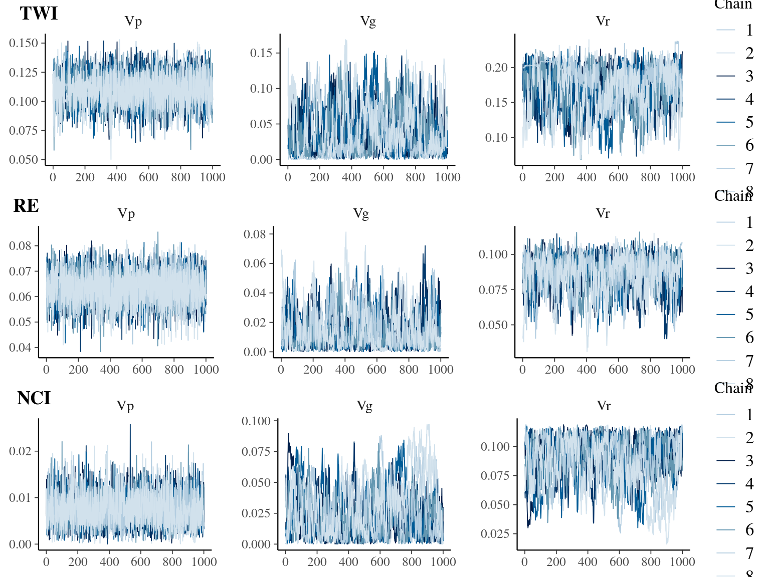
Figure 20.2: Traceplot for environmental variables.
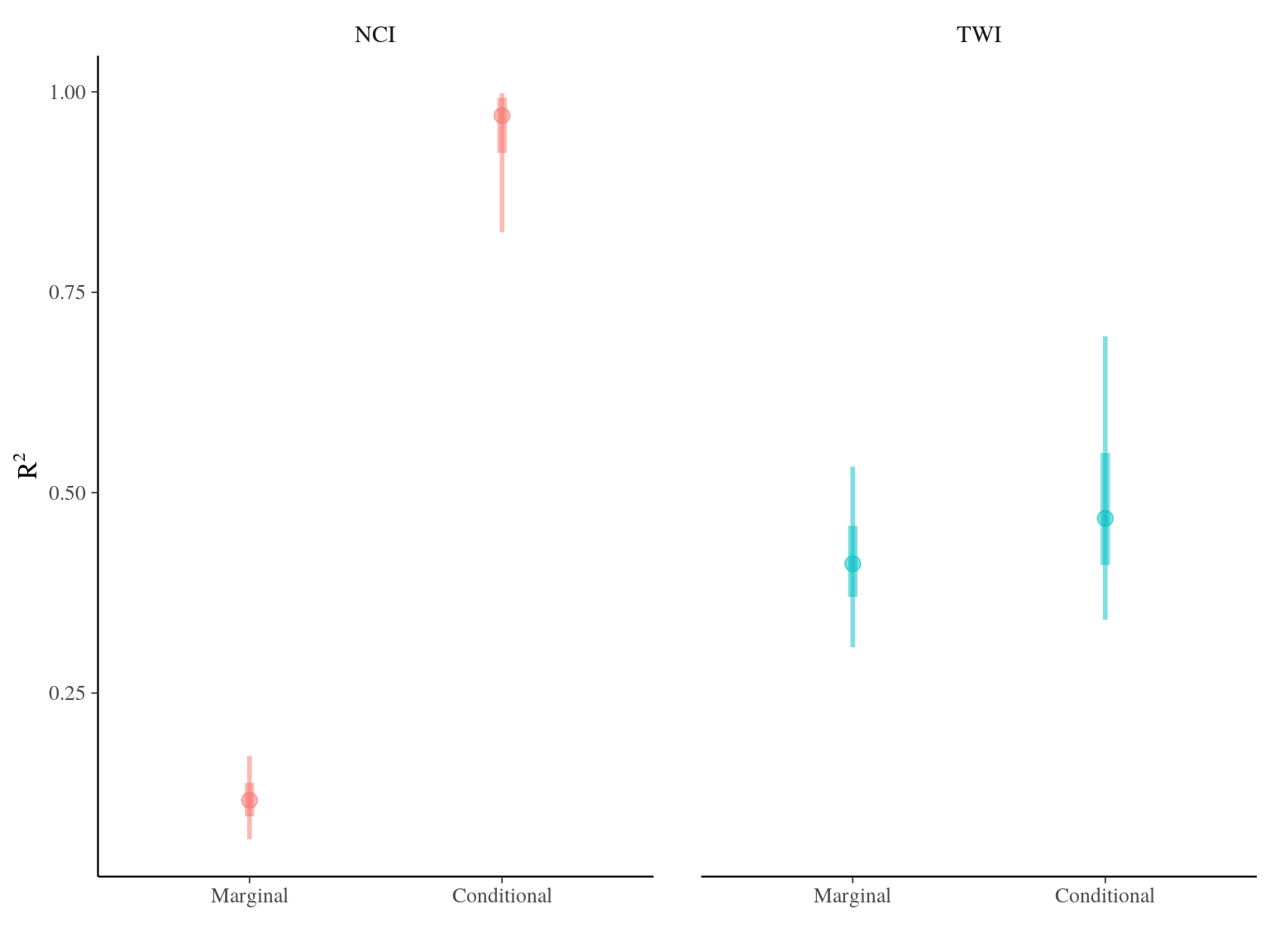
Figure 20.3: R2 for environmental variable
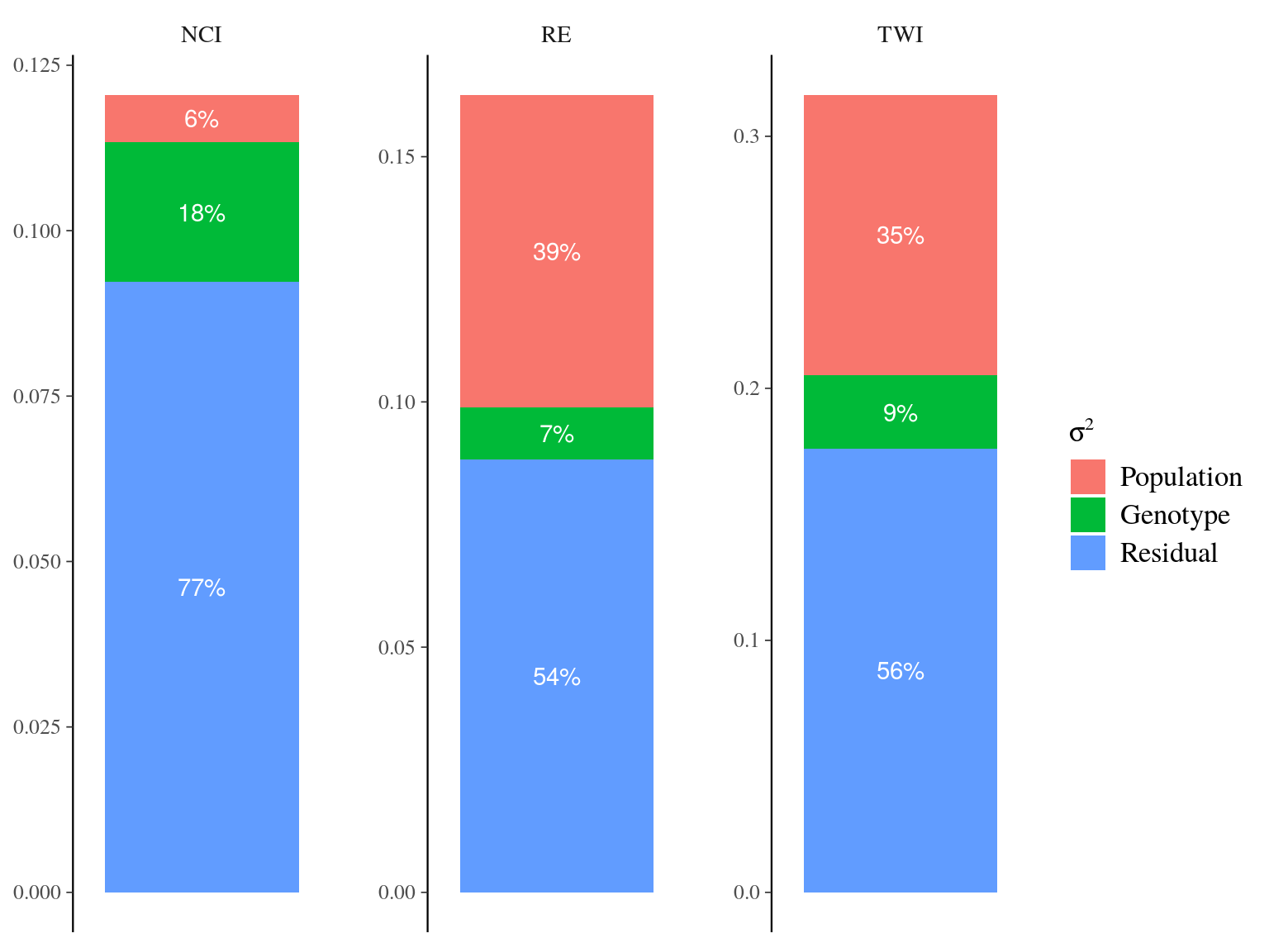
Figure 20.4: Genetic variance partitionning for environmental variables.
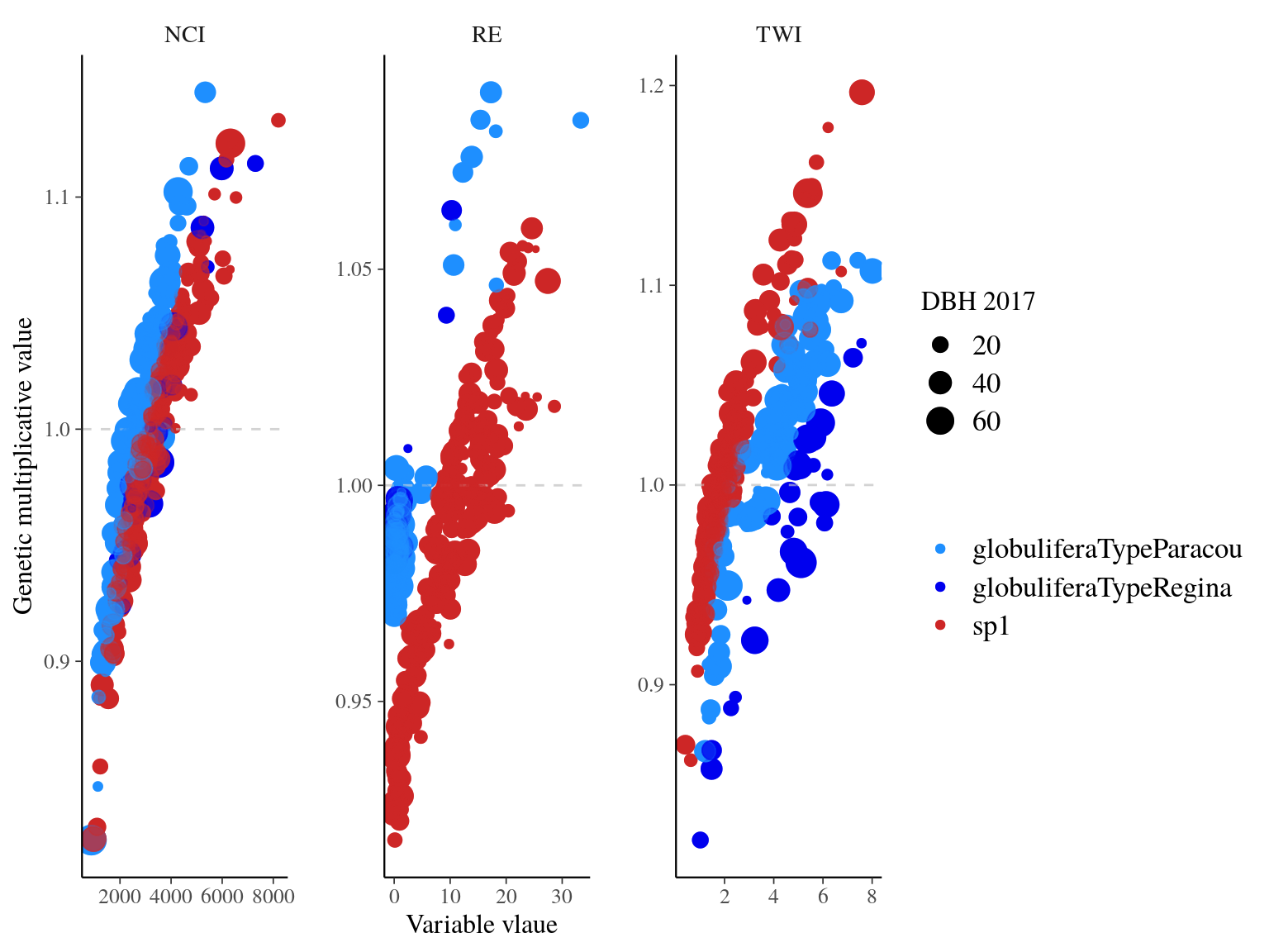
Figure 20.5: Multiplicative
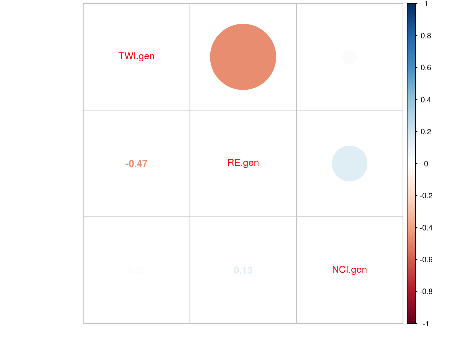
Figure 20.6: Multiplicative
20.3 Association
We used per SNP linear mixed models implemented in GEMMA (Genome-wide Efficient Mixed Model Analysis, Zhou & Stephens 2012) to identify major effect SNPs. Linear mixed models are calculated for the environemental values \(y\) of the \(N\) individuals with following formula:
\[\begin{equation} y_i \sim \mathcal N(\mu + x_i.\beta + Z.u_i, \sigma_E) \\ u_i \sim \mathcal{MVN_N}(0,\sigma_G.K) \\ \sigma_P = \sigma_G + \sigma_E \tag{20.4} \end{equation}\]
where \(N\) is the number of individuals, \(y\) is the vector of environmental variable values for the \(N\) individual, \(\mu\) is the intercept representing the mean environmental variable, \(x\) is a SNP, \(\beta\) is the effect size of the SNP, \(Z\) is the loading matrix (computed with Cholesky decomposition of \(K\)) and \(u\) is the vector of random effects corresponding to individuals kinship relations (\(u\) thus represents individuals breeding values), \(u\) values are centered on 0, covary with known kinship matrix \(K\) with an associated genetic variance \(\sigma_G\), \(\sigma_E\) is the residual variance, and the sum of residual \(\sigma_E\) and genetic \(\sigma_G\) variances is equal to the phenotypic variance \(\sigma_P\). \(\beta\) significance is calculated with Wald test. And p-values are corrected for multiple testing with false discovery rate, resulting in q-values.
Within each population, we didb’t detect any outliers SNPs both with TWI and NCI (Fig. 20.7).
module load bioinfo/plink-v1.90b5.3
module load bioinfo/gemma-v0.97
pops=(globuliferaTypeParacou globuliferaTypeRegina sp1)
for var in $(seq 2)
  do
  for pop in "${pops[@]}" ;
    do
      plink \
        --bfile env \
        --allow-extra-chr \
        --keep  $pop.fam \
        --extract env.prune.in \
        --maf 0.05 \
        --pheno env.phenotype --mpheno $var \
        --out $pop.var$var --make-bed ;
      gemma -bfile $pop.var$var -gk 1 -o kinship.$pop.var$var ;
      gemma -bfile $pop.var$var -lmm 1 \
        -k output/kinship.$pop.var$var.cXX.txt \
        -o LMM.$pop.var$var ;
  done
done
cat LMM.snps | cut -f1 > snps.list
plink --bfile env --allow-extra-chr --extract snps.list --out outliers --recode A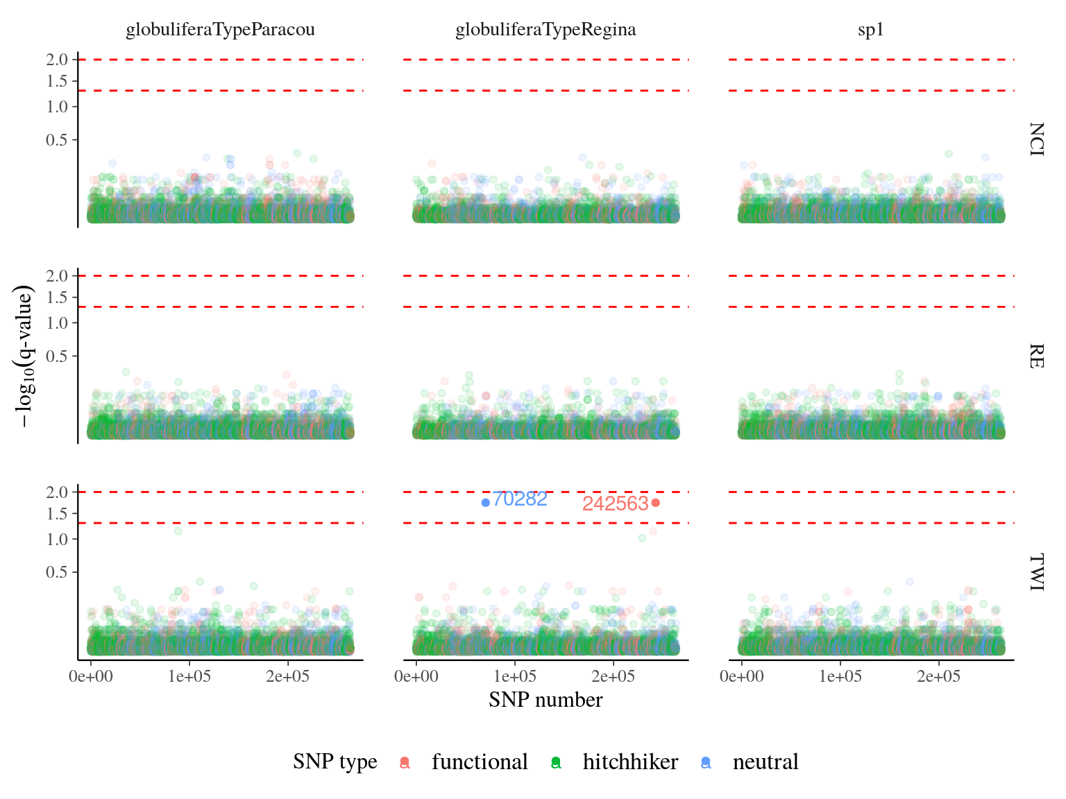
Figure 20.7: q-value of major effect SNPs associated to environmental variables. SNP were detected using linear mixed models (LMM) with individual kiniship as random effect. SNP significance was assessed with Wald test. q-value was obtained correcting mutlitple testing with false discovery rate.
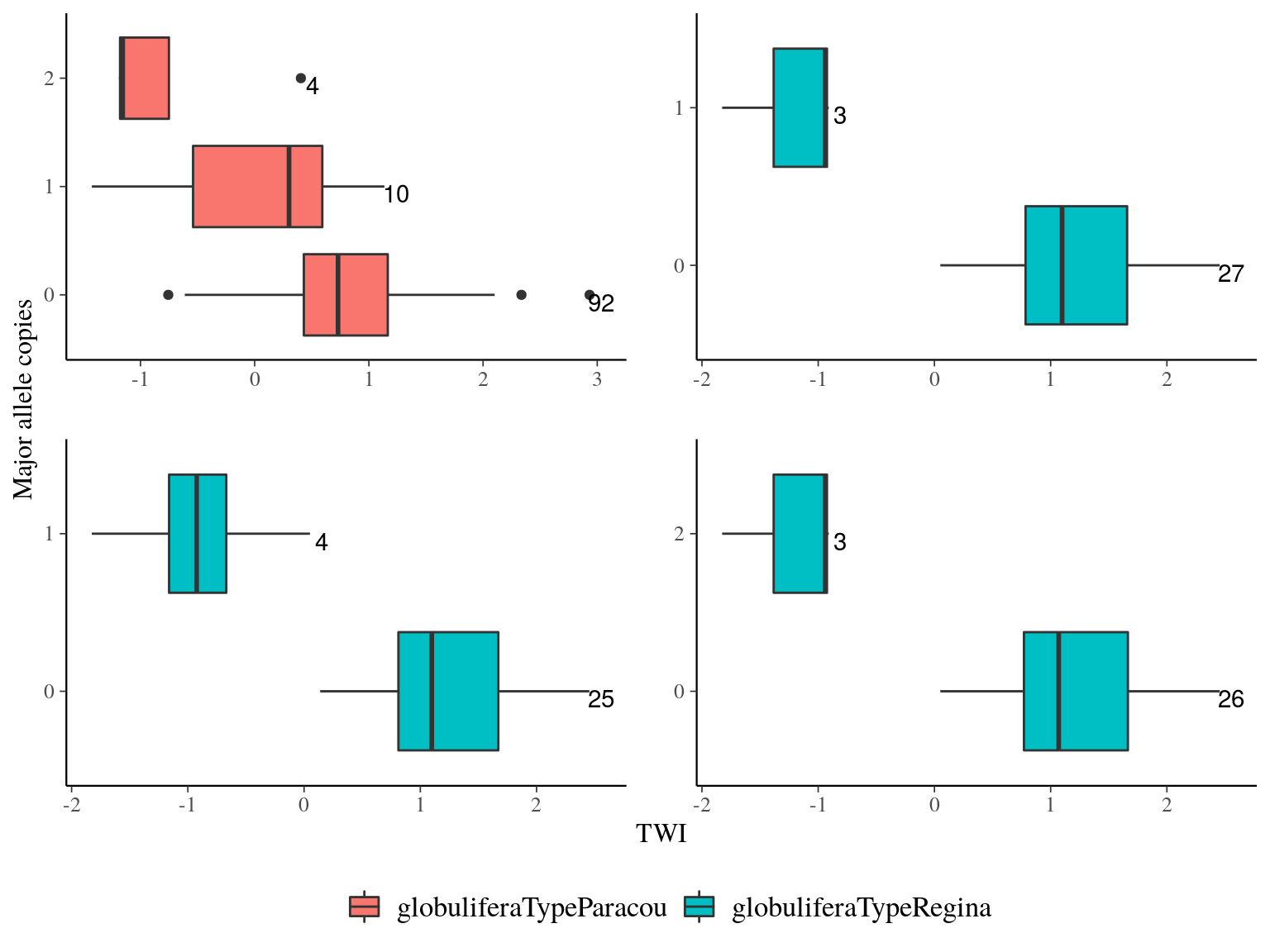
Figure 20.8: TWI distribution for outliers genes.
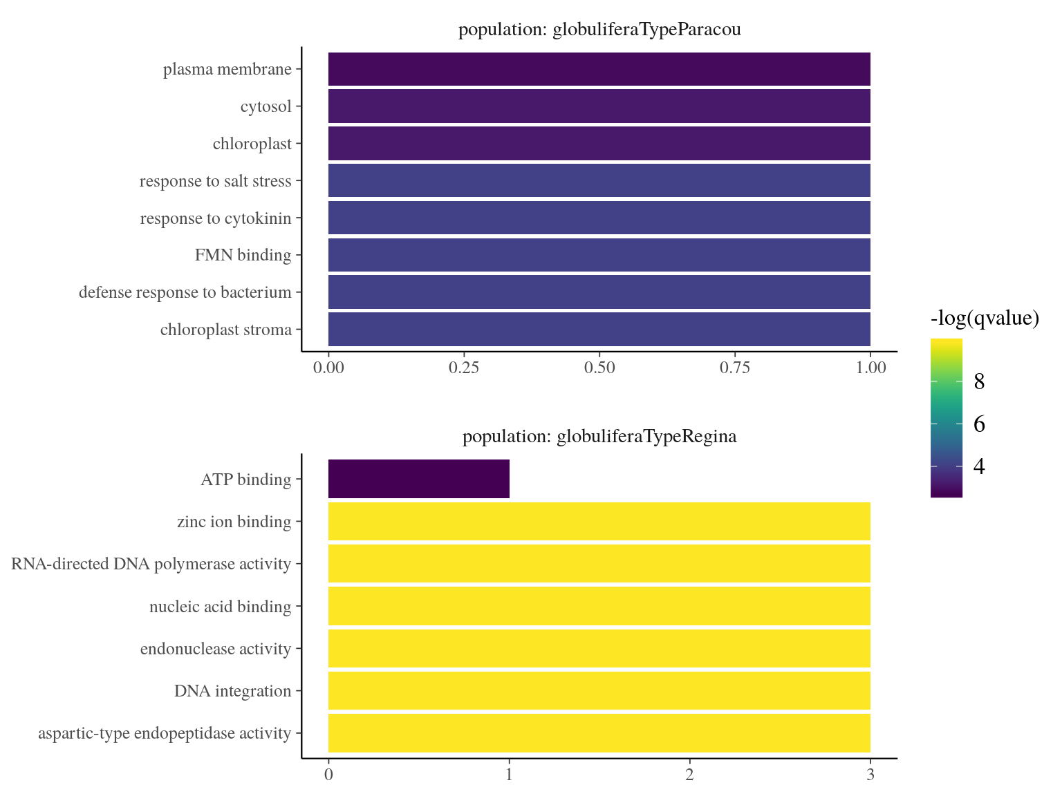
Figure 20.9: Term enrichment of Gene Ontology (GO) for outliers genes.
References
Allié, E., Pélissier, R., Engel, J., Petronelli, P., Freycon, V., Deblauwe, V., Soucémarianadin, L., Weigel, J. & Baraloto, C. (2015). Pervasive local-scale tree-soil habitat association in a tropical forest community. PLoS ONE, 10, 1–16.
Conrad, O., Bechtel, B., Bock, M., Dietrich, H., Fischer, E., Gerlitz, L., Wehberg, J., Wichmann, V. & Böhner, J. (2015). System for Automated Geoscientific Analyses (SAGA) v. 2.1.4. Geoscientific Model Development, 8, 1991–2007. Retrieved from https://www.geosci-model-dev.net/8/1991/2015/
Ferry, B., Morneau, F., Bontemps, J.-D., Blanc, L. & Freycon, V. (2010). Higher treefall rates on slopes and waterlogged soils result in lower stand biomass and productivity in a tropical rain forest. Journal of Ecology, 98, 106–116. Retrieved from http://doi.wiley.com/10.1111/j.1365-2745.2009.01604.x
Rellstab, C., Gugerli, F., Eckert, A.J., Hancock, A.M. & Holderegger, R. (2015). A practical guide to environmental association analysis in landscape genomics. 24, 4348–4370. Retrieved from http://doi.wiley.com/10.1111/mec.13322
Uriarte, M., Condit, R., Canham, C.D. & Hubbell, S.P. (2004). A spatially explicit model of sapling growth in a tropical forest: Does the identity of neighbours matter? Journal of Ecology, 92, 348–360. Retrieved from http://doi.wiley.com/10.1111/j.0022-0477.2004.00867.x
Wilson, A.J., Réale, D., Clements, M.N., Morrissey, M.M., Postma, E., Walling, C.A., Kruuk, L.E.B. & Nussey, D.H. (2010). An ecologist’s guide to the animal model. Journal of Animal Ecology, 79, 13–26. Retrieved from https://pdfs.semanticscholar.org/931b/921e07dc932e3f34e78bc3ca5a7bfe472e04.pdf
Zhou, X. & Stephens, M. (2012). Genome-wide efficient mixed-model analysis for association studies. Nature Genetics, 44, 821–824. Retrieved from http://www.nature.com/articles/ng.2310