Chapter 5 Fuctional region selection
We used open reading frames (ORF) to target genes within scaffolds. ORFs have been detected with transdecoder on assembled transcripts. First, we filtered ORFs including a start codon(figure 5.1). Then, we aligned ORFs on pre-selected and merged genomic scaffolds with blat. We obtained 7 744 aligned scaffolds (table 5.1 and figure 5.2). Thanks to the alignment, we removed overlapping genes (figure 5.3) and obtained 4 076 pre-selected genes with a total length of 757 hbp (figure 5.4). Finally we used transcript differential expression to select all genes differentially expressed between Symphonia globulifera and Symphonia sp1 (figure 5.5). We selected 1150 sequences of 500 to 1-kbp representing 1 063 Mbp (table 5.2). To validate our final target set, we aligned with bwa raw reads from one library from Scotti et al. (in prep). …
5.1 Open Reading Frames (ORFs) filtering
173 828 ORFs including a start codon (Methyonin, M) were detected (over 231 883, 75%, see figure 5.1.
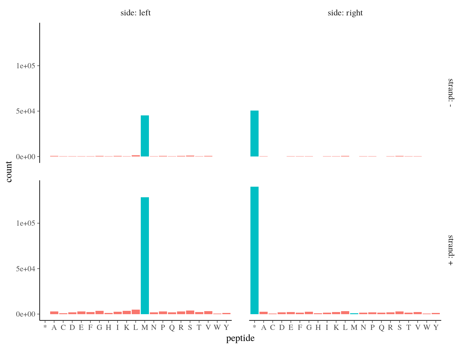
Figure 5.1: Open Reading Frames left and right peptides.
orf <- src_sqlite(file.path(path, "Niklas_transcripts/Trinotate/",
                           "symphonia.trinity500.trinotate.sqlite")) %>%
  tbl("ORF") %>%
  dplyr::rename(orf = orf_id, trsc = transcript_id,
                orfSize = length) %>%
  filter(substr(peptide, 1, 1) == "M") %>%
  select(-peptide, -strand) %>%
  collect() %>%
  rowwise() %>%
  mutate(orfStart = min(as.numeric(lend), as.numeric(rend)),
         orfEnd = max(as.numeric(lend), as.numeric(rend))) %>%
  select(-lend, -rend) %>%
  select(trsc, orfStart, orfEnd, orf) %>%
  mutate_if(is.numeric, as.character) %>%
  write_tsv(path = file.path(path, "functional_selection2", "orf.all.bed"),
            col_names = F)
5.2 ORF alignment on genomics scaffolds
7 744 scaffolds matched with ORFs (10.5% for 15.4 Mbp, see table 5.1 and figure 5.2).
cd ~/Documents/BIOGECO/PhD/data/Symphonia_Genomes/functional_selection2
cat orf.all.bed | sort -k 1,1 -k2,2n >  orf.all.sorted.bed
trsc=/home/sylvain/Documents/BIOGECO/PhD/data/Symphonia_Niklas/filtered_transcripts.fasta
bedtools getfasta -name -fi $trsc -bed orf.all.sorted.bed -fo orf.fasta
scf=~/Documents/BIOGECO/PhD/data/Symphonia_Genomes/neutral_selection/merged.fasta
orf=./orf.fasta
blat $scf $orf alignment.psl| N | Width (Mbp) | Coverage (%) | |
|---|---|---|---|
| aligned sequence | 21 146 | 2.201315 | 1.499565 |
| selected scaffold | 7 744 | 15.425248 | 10.507881 |
| total | 82 792 | 146.796946 | 100.000000 |
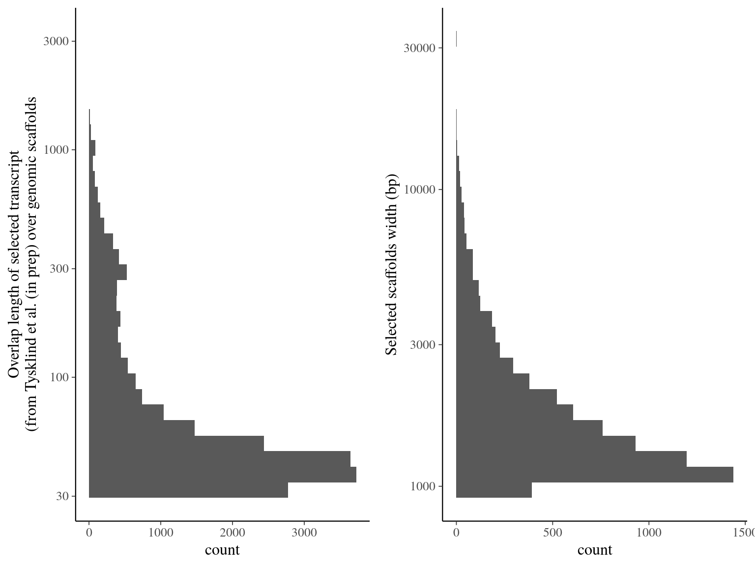
Figure 5.2: Alignment result of Tysklind et al. (in prep) ORFs over genomic scaffolds with blat. Left graph represents the overlap distribution. Right graph represent the selected and deduplicated scaffolds distribution.
5.3 Overlaping genes filtering
995 genes were overlapping and filtered out (figure 5.3).
alignment %>%
  separate(orf, into = c("gene", "isoform", "geneNumber", "orfNumber"),
           sep = "::", remove = F) %>%
  select(gene, orf, orfStart, orfEnd, scf, scfStart, scfEnd) %>%
  unique() %>%
  select(scf, scfStart, scfEnd, orf, gene) %>%
  arrange(scf, scfStart, scfEnd) %>%
  mutate_if(is.numeric, as.character) %>%
  write_tsv(path = file.path(path, "functional_selection2", "genes.all.bed"),
            col_names = F)
cd ~/Documents/BIOGECO/PhD/data/Symphonia_Genomes/functional_selection2
cat genes.all.bed | sort -k 1,1 -k2,2n > genes.all.sorted.bed
bedtools merge -i genes.all.sorted.bed -c 5 -o collapse > genes.merged.bed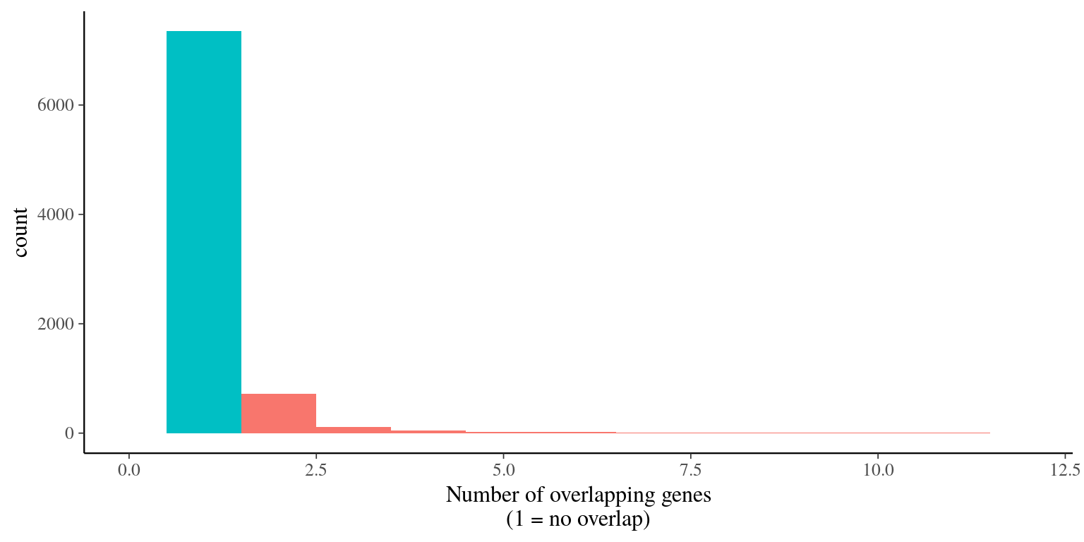
Figure 5.3: Genes overlap
5.4 Pre-selected genes
We obtained 4 076 genes pre-selected for a total length of 757 kbp (figure 5.4).
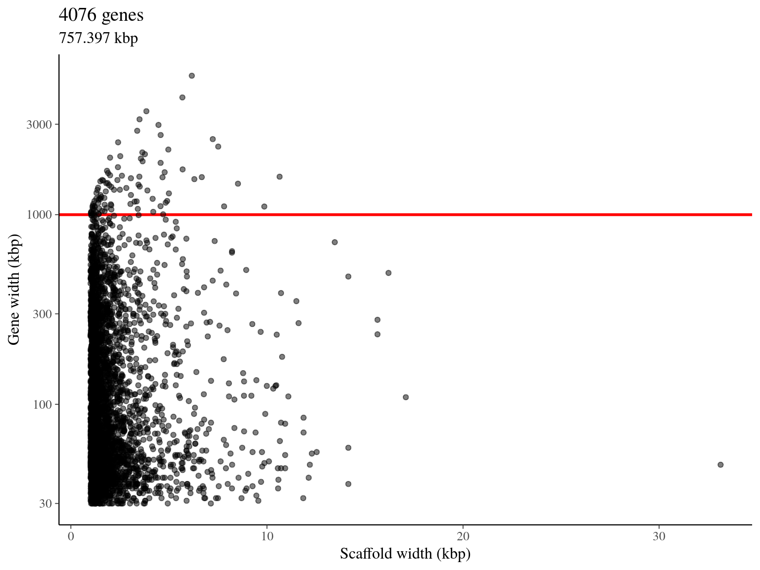
Figure 5.4: Available genes for target sequences design.
5.5 Differential Expression (DE) of genes
Figure 5.5 shows genes differential expression. First circle represent genes with isoforms not enriched whereas second and third circle represents respectivelly genes with isoforms S. sp1 and S. globulifera enriched. Relatively few genes contained enriched isoforms, and most of them were S. globulifera enriched.
Figure 5.5: Genes differential expression.
5.6 Final subset of selected functional scaffolds
We finally selected 1150 sequences of 500 to 1-kbp with 100 bp before geneStart and a maximum of 900 bp after, resulting in 1 063, 544 kbp of targets. All differentially expressed genes between morphotypes were selected (159). And the rest of sequences were selected among non differentially expressed genes randomly (1001).
targets <- genes %>%
  left_join(de) %>%
  filter(deg %in% c("Eglo", "Esp")) %>%
  rbind(genes %>%
          left_join(de) %>%
          filter(deg %in% c("DE", NA)) %>%
          sample_n(1309)) %>%
  group_by(scf, gene) %>%
  filter(n() < 2) %>%
  mutate(targetStart = max(0, geneStart - 100)) %>%
  mutate(targetEnd = min(targetStart + 1000, scfSize)) %>%
  mutate(targetSize = targetEnd - targetStart) %>%
  filter(targetSize > 500) %>%
  mutate(target = paste0(gene, "_on_", scf)) %>%
  ungroup()
targets %>%
  select(scf, targetStart, targetEnd, target) %>%
  arrange(scf, targetStart, targetEnd, target) %>%
  mutate_if(is.numeric, as.character) %>%
  write_tsv(path = file.path(path, "functional_selection2", "targets.all.bed"),
            col_names = F)
cd ~/Documents/BIOGECO/PhD/data/Symphonia_Genomes/functional_selection2
cat targets.all.bed | sort -k 1,1 -k2,2n > targets.all.sorted.bed
scf=~/Documents/BIOGECO/PhD/data/Symphonia_Genomes/neutral_selection/merged.fasta
bedtools getfasta -name -fi $scf -bed targets.all.sorted.bed -fo targets.fasta| N | Width (Mbp) | Mask (%N) |
|---|---|---|
| 1 165 | 1.068207 | 0.0025285 |
5.7 Repetitive regions final check
Last but not least, we do not want to include repetitive regions in our targets for baits design. We consequently aligned raw reads from one library from Scotti et al. (in prep) on our targets with bwa.
cd ~/Documents/BIOGECO/PhD/data/Symphonia_Genomes/functional_selection2
reference=targets.fasta
query=~/Documents/BIOGECO/PhD/data/Symphonia_Genomes/Ivan_2018/raw_reads/globu1_symphonia_globulifera_CTTGTA_L001_R1_001.fastq.gz
bwa index $reference
bwa mem -M $reference $query > raw_read_alignment.sam
picard=~/Tools/picard/picard.jar
java -Xmx4g -jar $picard SortSam I=raw_read_alignment.sam O=raw_read_alignment.bam SORT_ORDER=coordinate
bedtools bamtobed -i raw_read_alignment.bam > raw_read_alignment.bed
cat raw_read_alignment.bed | sort -k 1,1 -k2,2n >  raw_read_alignment.sorted.bed
bedtools merge -i raw_read_alignment.sorted.bed -c 1 -o count > raw_read_alignment.merged.bed
We obtained a continuous decreasing distribution of read coverage across our scaffolds regions (figure 5.6). We fitted a \(\Gamma\) distribution with positive parameters for scaffolds regions with a coverage under 5 000 (non continuous distribution with optimization issues). We obtained a distribution with a mean of 309 reads per region and a \(99^{th}\) quantile of 2 606. We decided to mask regions with a coverage over the \(99^{th}\) quantile and remove scaffolds with a mask superior to 75% of its total length (figure ??).
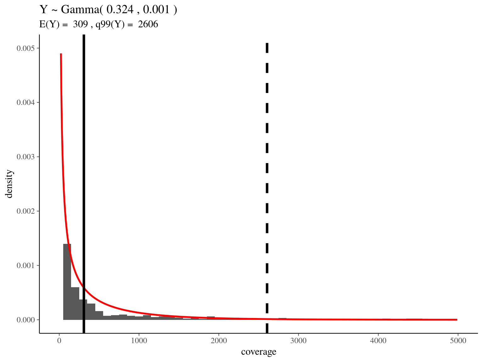
Figure 5.6: Read coverage distribution.
repetitive_target <- bed %>%
  filter(coverage > qgamma(0.99, alpha, beta)) %>%
  mutate(size = end - start)
repetitive_target %>%
  select(target, start, end) %>%
  arrange(target, start, end) %>%
  mutate_if(is.numeric, as.character) %>%
  write_tsv(path = file.path(path, "functional_selection2", "repetitive_targets.bed"),
            col_names = F)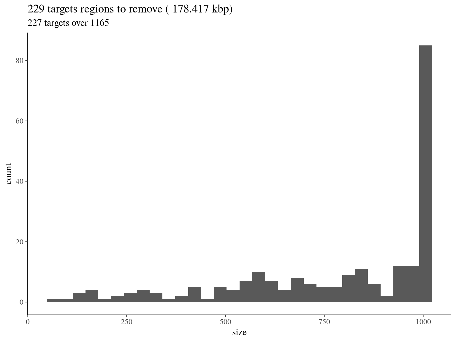
Figure 5.7: target regions with a coverage over the 99th quantile of the fitted Gamma distribution (2606).
cd ~/Documents/BIOGECO/PhD/data/Symphonia_Genomes/functional_selection2
cat repetitive_targets.bed | sort -k 1,1 -k2,2n >  repetitive_targets.sorted.bed
bedtools maskfasta -fi targets.fasta -bed repetitive_targets.sorted.bed -fo targets.masked.fasta
targets <- readDNAStringSet(file.path(path, "functional_selection2", "targets.masked.fasta"))
writeXStringSet(targets[which(letterFrequency(targets, "N")/width(targets) < 0.65)],
file.path(path, "functional_selection2", "targets.filtered.masked.fasta"))| N | Width (Mbp) | Mask (%N) |
|---|---|---|
| 975 | 0.896759 | 0.0168273 |