Chapter 10 Capture
We will do 16 reactions of gene capture by hybridization. Each reaction can have up to 32 samples. We will proceed as follow:
- Amplifcation 1 Plate reorganization: plates state and volme will be assessed and 6 new plates (P1 to P6) will be build from (i) original libraries (P1-P5), (ii) reamplified libraries (A1-A2), and (iii) extraction and library repeat (P6). In order to do so, P6 will stay unchanged, and new plate 1 to 5 will be either reamplified libraries or original libraries if not reamplified. Tip: remove unwanted cone from boxes when transfering original P1 to P5 to new ones to work with multi-channel pipette and prepare correspondance table to transfer reamplified plates A1 and A2 to new P1 to P5 plates crossing each line one-by-one.
- DNA dosage 1: with PicoGreen, we will assess DNA concentration of each sample with a lader from 5 to 30 \(ng.\mu L^{-1}\) in order to correctly dose low concentration samples. Tip: PicoGreen have to be used before the 26/03 12h or after the 1/04.
- Amplification 2: Samples that have never been reamplified with a concentration below 1 \(ng.\mu L^{-1}\) will be reorganized on a new plate (A3) and reamplified with 8 cycles.
- DNA dosage 2: Re-amplified samples (A3) will be dosed through NanoDrop and other more accurate technology depending on the availability.
- Amplifcation 2 and Library Repeat Plates reorganization: Re-amplified samples (A3) will be redistributed in their original position within library plates, and plates and 6.2 will be reorganized in a unique plate 6.3 for pools building.
- Pool building: Pool building will follow plate organization, with re-extracted samples (P6.2) pooled together due to high fragmet size heterogeneity. Pool building must be equimolar and will thus depend on DNA dosage. Because we won’t pipette less than 0.5 \(\mu L\) of the most concentrated sample of one pool, depending on the concetration of the less concentrated sample, we might need to do dilution.
- Purification & Concentration: AMPure beads will be used to clean pools. We will also use this step to concentrate samples in a smaller volume for the reaction (targeted volume of reaction is 7 \(\mu L\) with 100 to 500 \(ng\) of DNA).
- Size assessment: Pools fragments size will be assessed with TapeStation, in order to check for correct fragment size distribution, and eventuelly further clean library pools.
- Size selection: if size distribution result is not good enough, we will further clean library pools through size selection with a Pippin. Info: we thus avoid capture fail with too small fragments but we risk losing libraries.
- Capture: Finally we realized capture by hybridization following ArborScience protocol
10.1 Amplifcation 1 Plate reorganization
First amplification plates (A1 and A2) have been redistributed within their original library plates removing previous libraries.
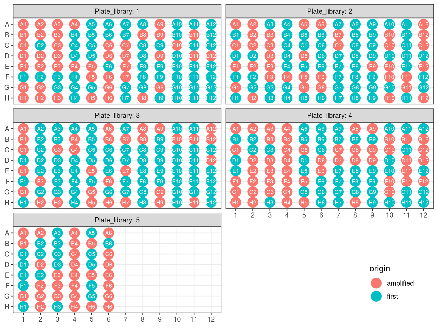
Figure 10.1: Original libraries to be kept (P1-P5).
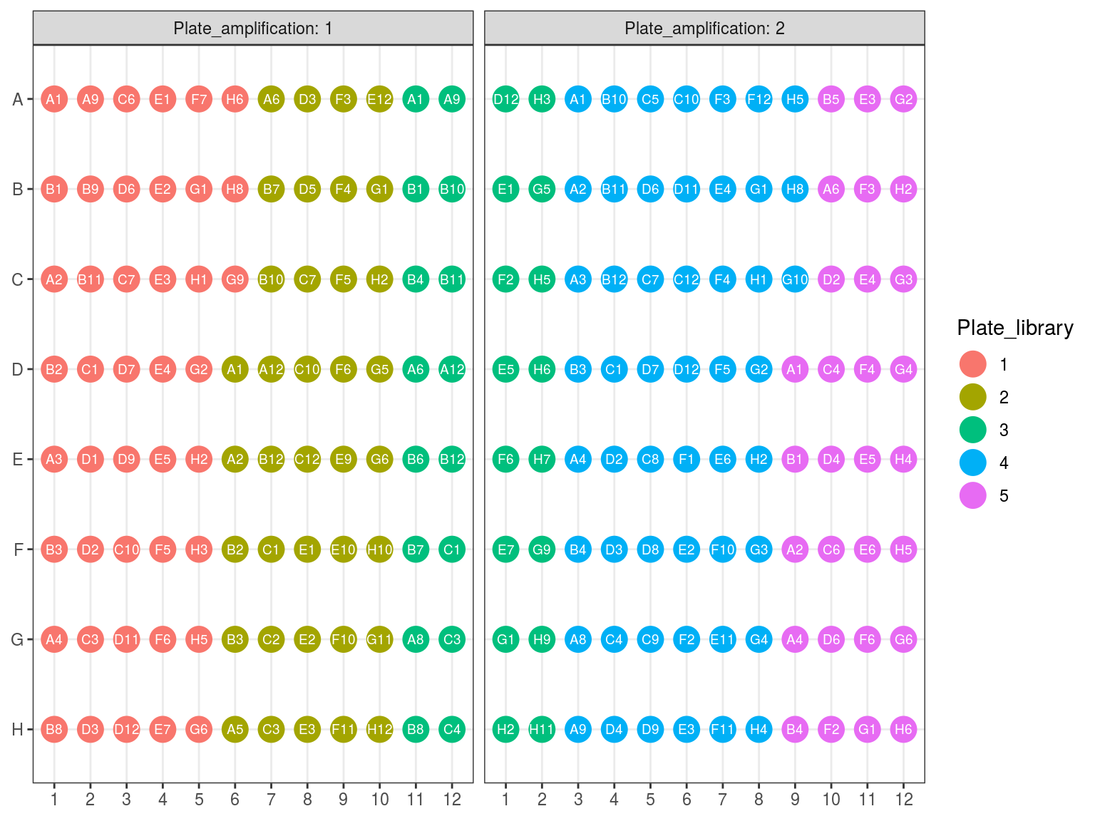
Figure 10.2: Original position of amplified samples.
10.2 DNA dosage 1
Samples concentration has been assessed by PicoGreen with ca 60 samples having a concentration below \(1 ng.\mu L^{-1}\) among which 50 have not been reamplified (34 among original libraries, and the rest among repeated libraries or extractions). Those samples will be reamplified.
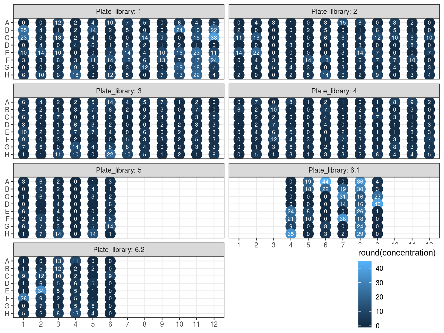
Figure 10.3: Sampled dosage by PicoGreen (concetration in ng.uL).
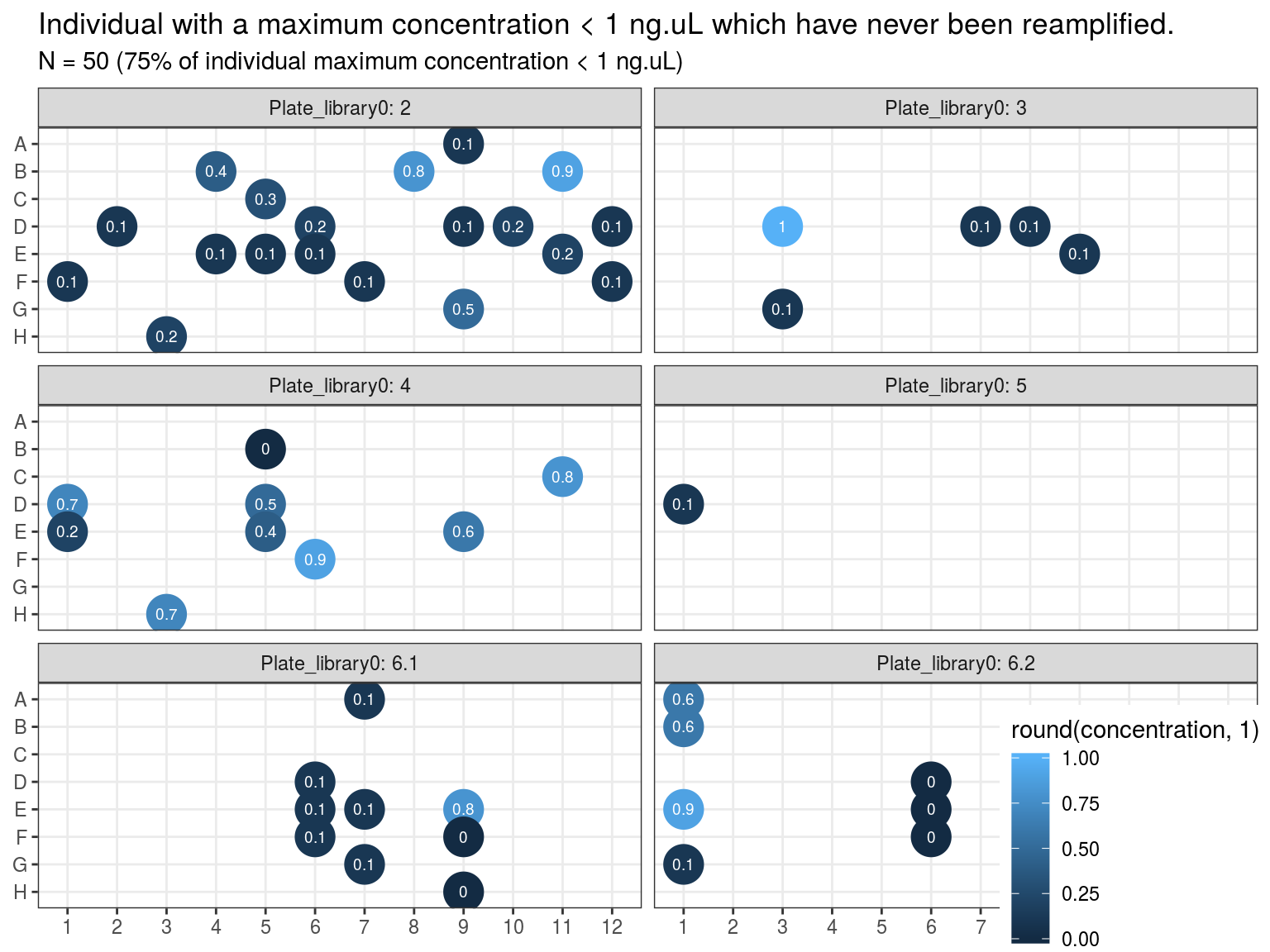
Figure 10.4: Samples to be re-amplified.
10.3 Amplification 2
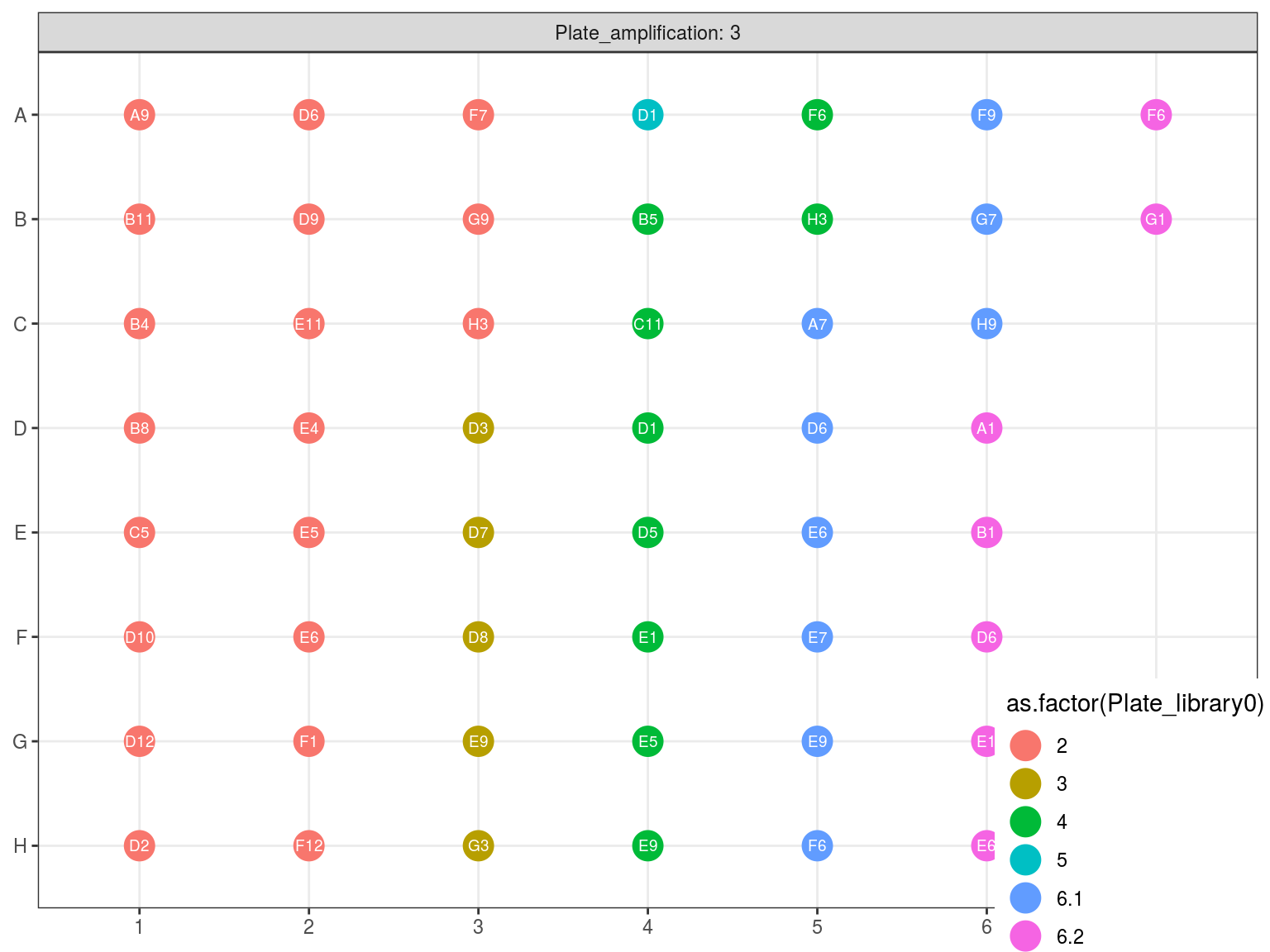
Figure 10.5: Original position of amplified samples in A3.
10.4 DNA dosage 2
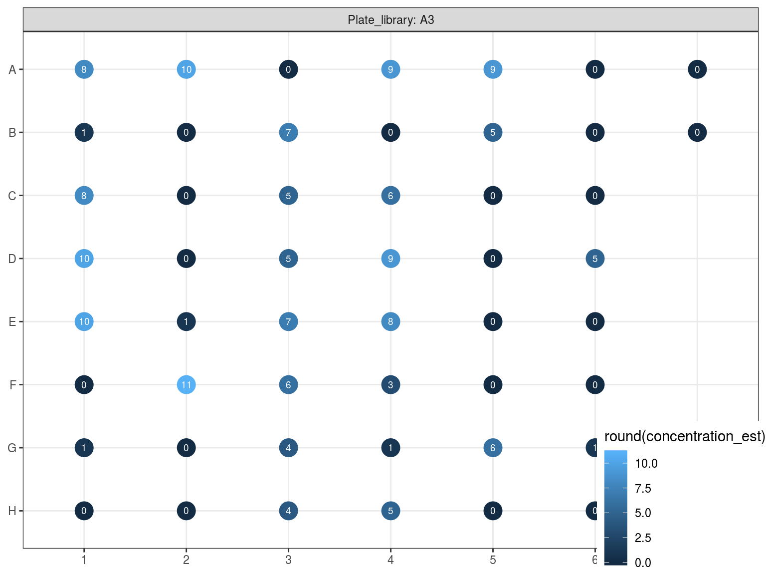
Figure 10.6: Reampified sampled dosage by PicoGreen (concetration in ng.uL).
10.5 Amplifcation 2 and Library Repeat Plates reorganization
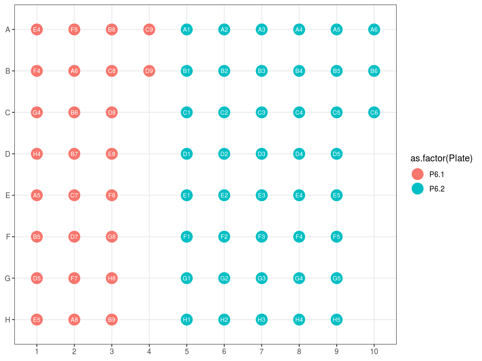
Figure 10.7: Original position of plate 6.1 and 6.2 reorganization in 6.3.
10.6 Pool building
Due to non uniformity of fragment size re-extracted samples from P6 (P6.2) will be treated in a single separated reaction (so 15 remainings). All other samples will be pulled by batch of 32 following plate order. We want 100 to 500 ng of DNA per reaction, and the reaction with the least samples have 16 samples. Consequently we will use 15 ng of each sample, resulting in 240 to 645 ng of DNA per sample (but we may lost material in purification, so we should aim for extra). Samples reaching to high concentration, for which we should sample less than 0.5 \(\mu L\) will be diluted 2 to 4 times.
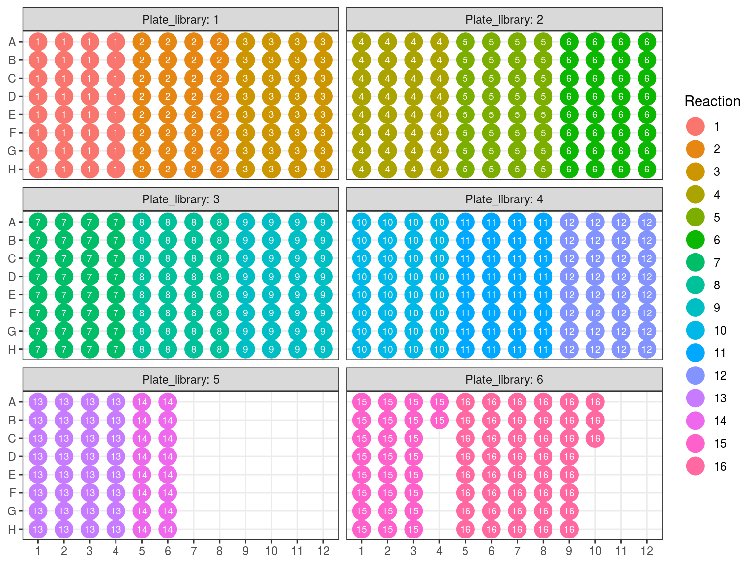
Figure 10.8: Sample reaction tube per plate.
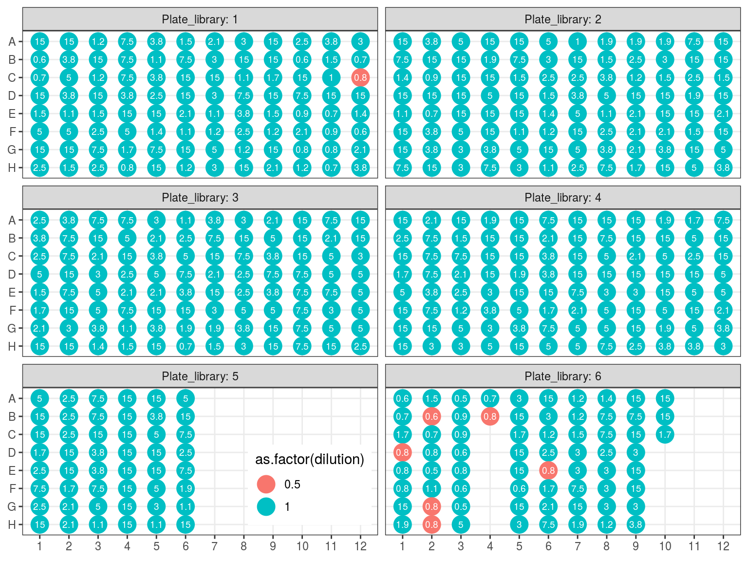
Figure 10.9: Sample reaction volume per plate.
10.7 Purification & Concentration
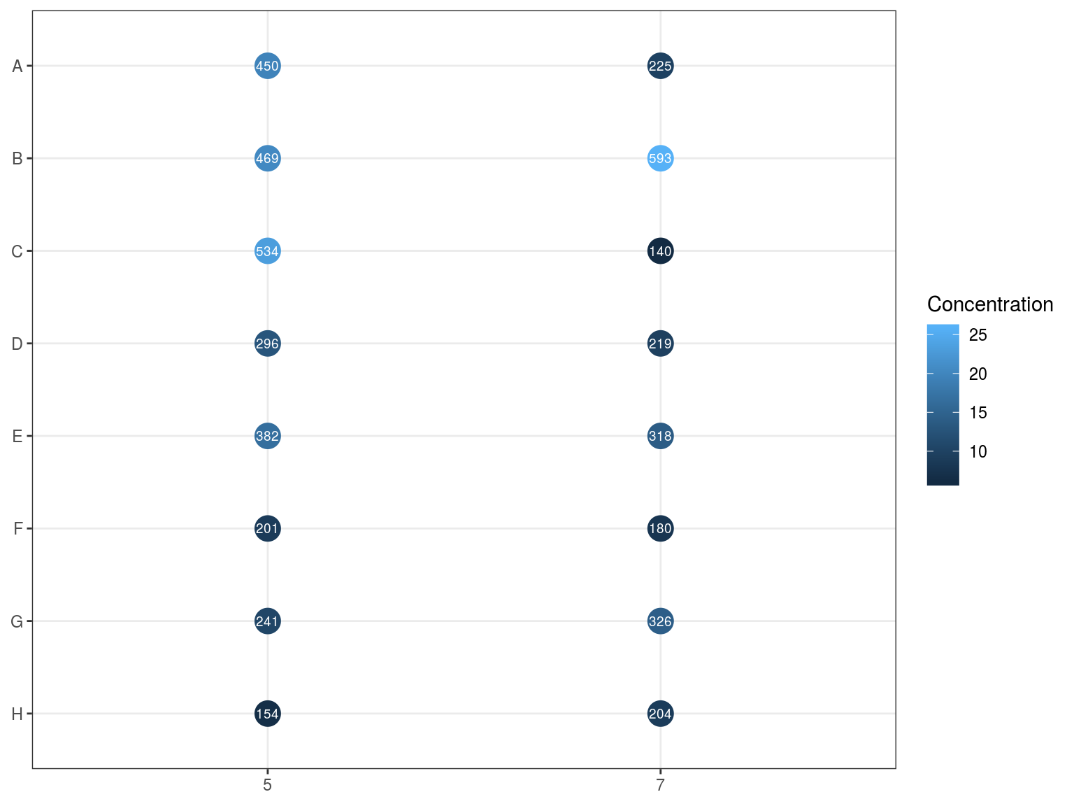
Figure 10.10: Reactions DNA content assessed by NanoDrop.
10.8 Size assessment
We have an heterogeneity of ffragments size distribution among pools with a large spectrum (Fig. 10.11). We will use TapeStation to select fragments between 330 and 700 bp.
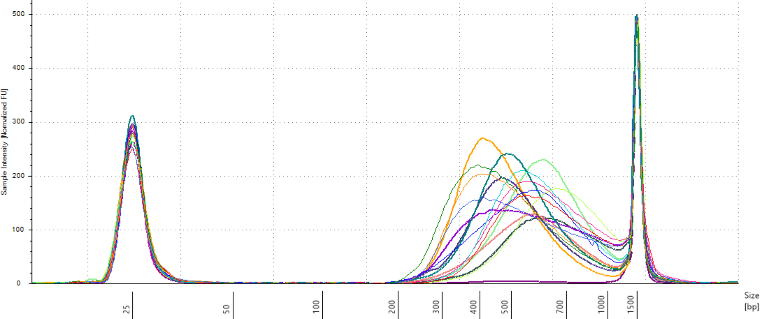
Figure 10.11: Pools size assessment.
10.9 Size selection
We will do pools of pools for the size selection with Pippin (Fig. 10.12), resulting in \(22*4=88 \mu L\) per pool. But the Pippin uses 30 \(\mu L\) and we want to do two reactions of Pippin per pool. So we reduced pool volume to 60 \(\mu L\) per pool with the speed vac. Then we used Pippin with a repeat of the 4 pools with 30 \(\mu L\) per pool. We used Pippin to filter fragments between 330 and 750 bp. After the Pippin, we cleaned the sampled with 1.8X PGTB Beads from Batch J, and assessed their concentration with QuBIT and their fragment size distribution with TapeStation. We obtained between 180 and 280 ng of DNA (Table 10.1) with fragments distributed between 300 and 700 bp (Fig. 10.13).
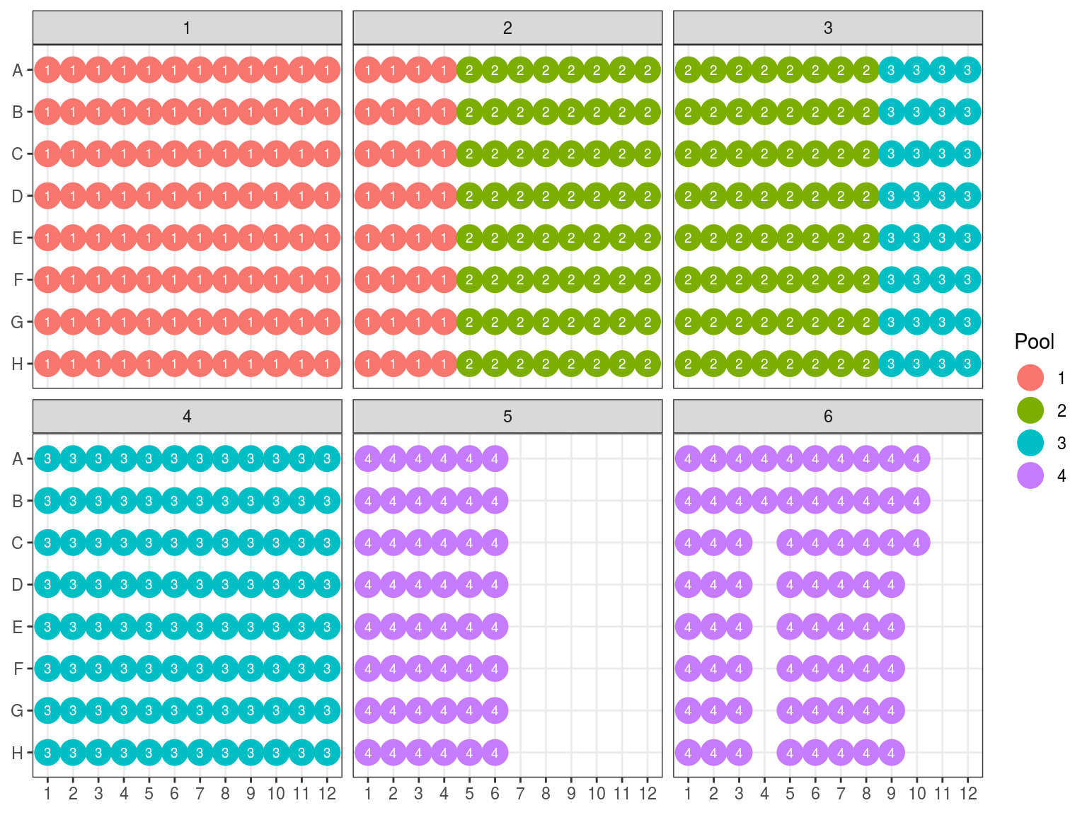
Figure 10.12: Pool of reactions.
| Pool | Repetition | Volume (\(\mu L\)) | Concentration (\(ng. \mu L^{-1}\)) | DNA (\(ng\)) | DNA origin (\(ng\)) | Loss factor |
|---|---|---|---|---|---|---|
| 1 | 1 | 37 | 4.94 | 182.78 | 874.0 | 5 |
| 2 | 1 | 37 | 5.33 | 197.21 | 489.0 | 2 |
| 3 | 1 | 37 | 7.38 | 273.06 | 588.5 | 2 |
| 4 | 1 | 37 | 3.98 | 147.26 | 514.0 | 3 |
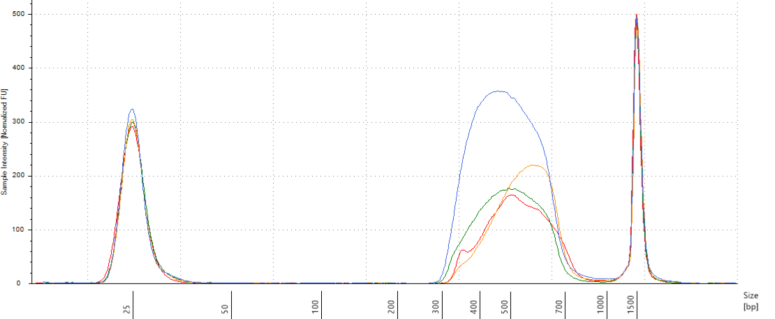
Figure 10.13: Size selected pools assessment.
10.10 Capture
We split the 4 pools in 16 reactions (4 replicates for each) and realized the capture following ArborScience protocol. After amplification we obtained between 227 and 987 ng of DNA per pool assessed by Qubit (with the four replicates summed, Table 10.2). We then pooled back the reaction, assessed their concentration by qPCR and adjust final samples for sequencing by an equimolar pooling Pool 1 and 2 and 3 and 4 togethers. We thus obtained 22 \(\mu L\) of Lane 1 at \(7.19~nM\) and 19 \(\mu L\) of Lane 2 at \(10.18~nM\) (see google sheets for more details). The material has been sent to Genotoul Get team for sequencing on Illumina HiSeq 3000 on two lanes of pair-ends 150 bp sequences.
| Reaction | Pool | Concentration (\(ng. \mu L^{-1}\)) | DNA (\(ng\)) | DNA pool (\(ng\)) |
|---|---|---|---|---|
| 1 | 1 | 11.300 | 440.700 | 957.450 |
| 2 | 1 | 5.850 | 228.150 | 957.450 |
| 3 | 1 | 5.500 | 214.500 | 957.450 |
| 4 | 1 | 1.900 | 74.100 | 957.450 |
| 5 | 2 | 1.250 | 48.750 | 242.775 |
| 6 | 2 | 1.075 | 41.925 | 242.775 |
| 7 | 2 | 2.350 | 91.650 | 242.775 |
| 8 | 2 | 1.550 | 60.450 | 242.775 |
| 9 | 3 | 7.350 | 286.650 | 986.700 |
| 10 | 3 | 5.650 | 220.350 | 986.700 |
| 11 | 3 | 5.800 | 226.200 | 986.700 |
| 12 | 3 | 6.500 | 253.500 | 986.700 |
| 13 | 4 | 1.380 | 53.820 | 227.955 |
| 14 | 4 | 1.095 | 42.705 | 227.955 |
| 15 | 4 | 1.935 | 75.465 | 227.955 |
| 16 | 4 | 1.435 | 55.965 | 227.955 |
\[ C~in~nM = \frac{C~in~ng/\mu L}{660 .average~fragment~size}.10^6\]
Dilution for qPCR (1 pM) Dilute in cascade your samples from 20.4 - 4.9 nM to almost 1 pM. So we need a 10 000 times dilution. We will do 4 1:10 dilutuions with \(1 \mu L\) of sample in \(9 \mu L\) of \(H_2O~miliQ\). Change of tips for every step and better use pipette in the middle of their range than in their extreme (e.g. for \(100 \mu L\) better use a \(200 \mu L\) than a \(100 \mu L\) pipette).