Chapter 22 Growth genomics

22.1 Gmax

We used the following growth model with a lognormal distribution to estimate individual growth potential:

\[\begin{equation} DBH_{y=today,p,i} - DBH_{y=y0,p,i} \sim \\ \mathcal{logN} (log(\sum _{y=y_0} ^{y=today} \theta_{1,p,i}.exp(-\frac12.[\frac{log(\frac{DBH_{y,p,i}}{100.\theta_{2,p}})}{\theta_{3,p}}]^2)), \sigma_1) \\ \theta_{1,p,i} \sim \mathcal {logN}(log(\theta_{1,p}), \sigma_2) \\ \theta_{2,p} \sim \mathcal {logN}(log(\theta_2),\sigma_3) \\ \theta_{3,p} \sim \mathcal {logN}(log(\theta_3),\sigma_4) \tag{22.1} \end{equation}\]

We fitted the equivalent model with following priors:

\[\begin{equation} DBH_{y=today,p,i} - DBH_{y=y0,p,i} \sim \\ \mathcal{logN} (log(\sum _{y=y_0} ^{y=today} \hat{\theta_{1,p,i}}.exp(-\frac12.[\frac{log(\frac{DBH_{y,p,i}}{100.\hat{\theta_{2,p}}})}{\hat{\theta_{3,p}}}]^2)), \sigma_1) \\ \hat{\theta_{1,p,i}} = e^{log(\theta_{1,p}) + \sigma_2.\epsilon_{1,i}} \\ \hat{\theta_{2,p}} = e^{log(\theta_2) + \sigma_3.\epsilon_{2,p}} \\ \hat{\theta_{3,p}} = e^{log(\theta_3) + \sigma_4.\epsilon_{3,p}} \\ \epsilon_{1,i} \sim \mathcal{N}(0,1) \\ \epsilon_{2,p} \sim \mathcal{N}(0,1) \\ \epsilon_{3,p} \sim \mathcal{N}(0,1) \\ ~ \\ (\theta_{1,p}, \theta_2, \theta_3) \sim \mathcal{logN}^3(log(1),1) \\ (\sigma_1, \sigma_2, \sigma_3, \sigma_4) \sim \mathcal{N}^4_T(0,1) \\ ~ \\ V_P = Var(log(\mu_p)) \\ V_R=\sigma_2^2 \tag{22.2} \end{equation}\]

Table 22.1: Individual growth potential model.
Parameter	Estimate	Standard error	\(\hat R\)	\(N_{eff}\)
thetap1[1]	0.5369487	0.0558649	1.052157	208
thetap1[2]	0.5418062	0.0975853	1.014136	304
thetap1[3]	0.3671035	0.0243181	1.033224	229
theta2	0.2545044	0.0806695	1.011055	702
theta3	0.7014813	0.1053930	1.020937	491
sigma[1]	0.1335699	0.0941555	1.508783	22
sigma[2]	0.6703421	0.0406016	1.141318	62
sigma[3]	0.2739054	0.2875370	1.007774	972
sigma[4]	0.1336316	0.2239892	1.008755	1160
lp__	362.3623923	267.2329411	1.741902	17

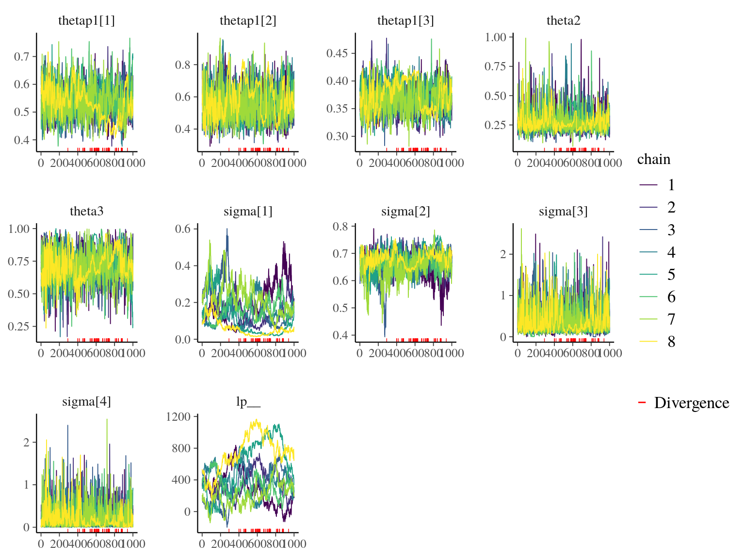
Figure 22.1: Traceplot of model parameters.

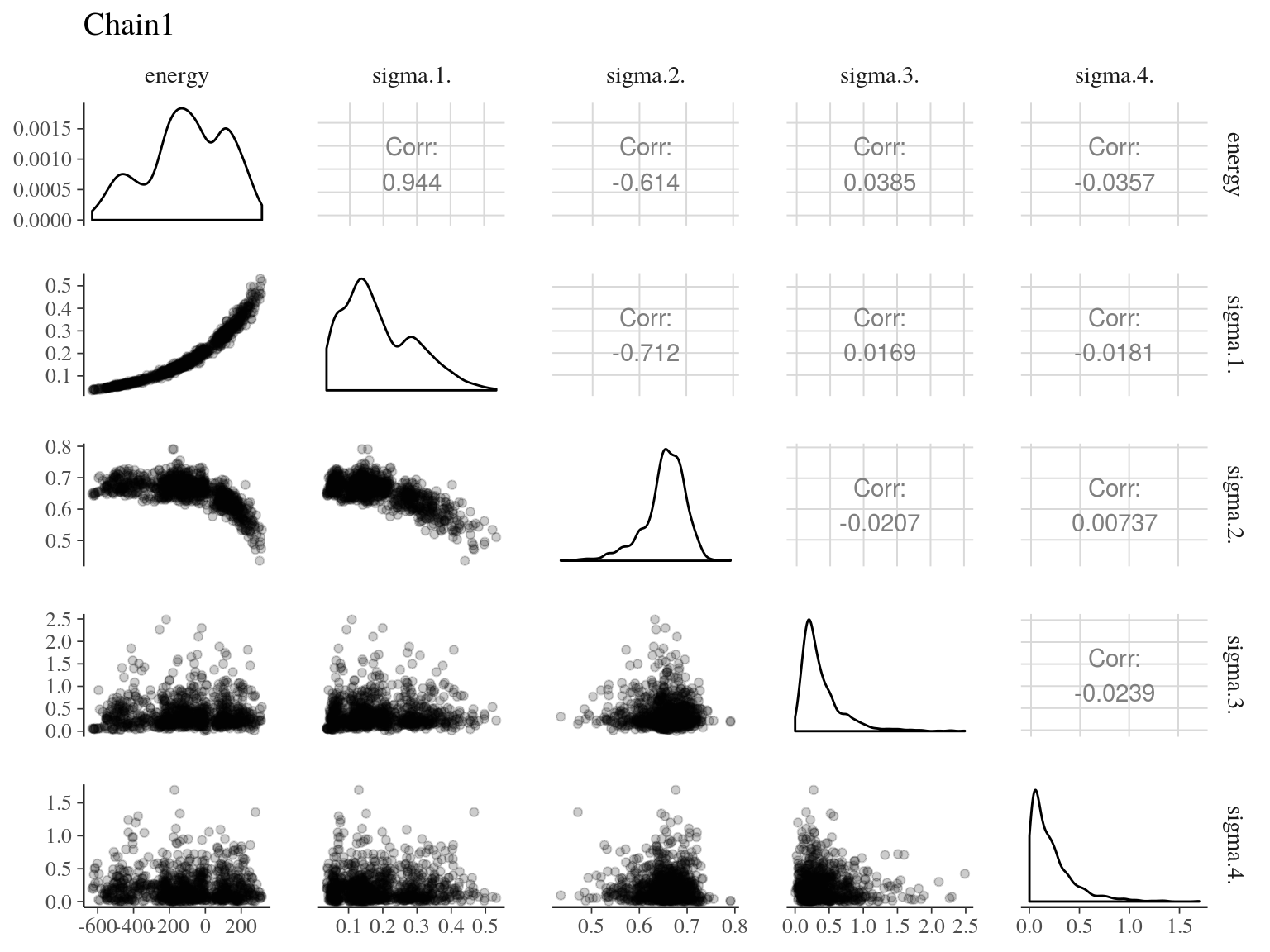
Figure 22.2: Pairs of model parameters.

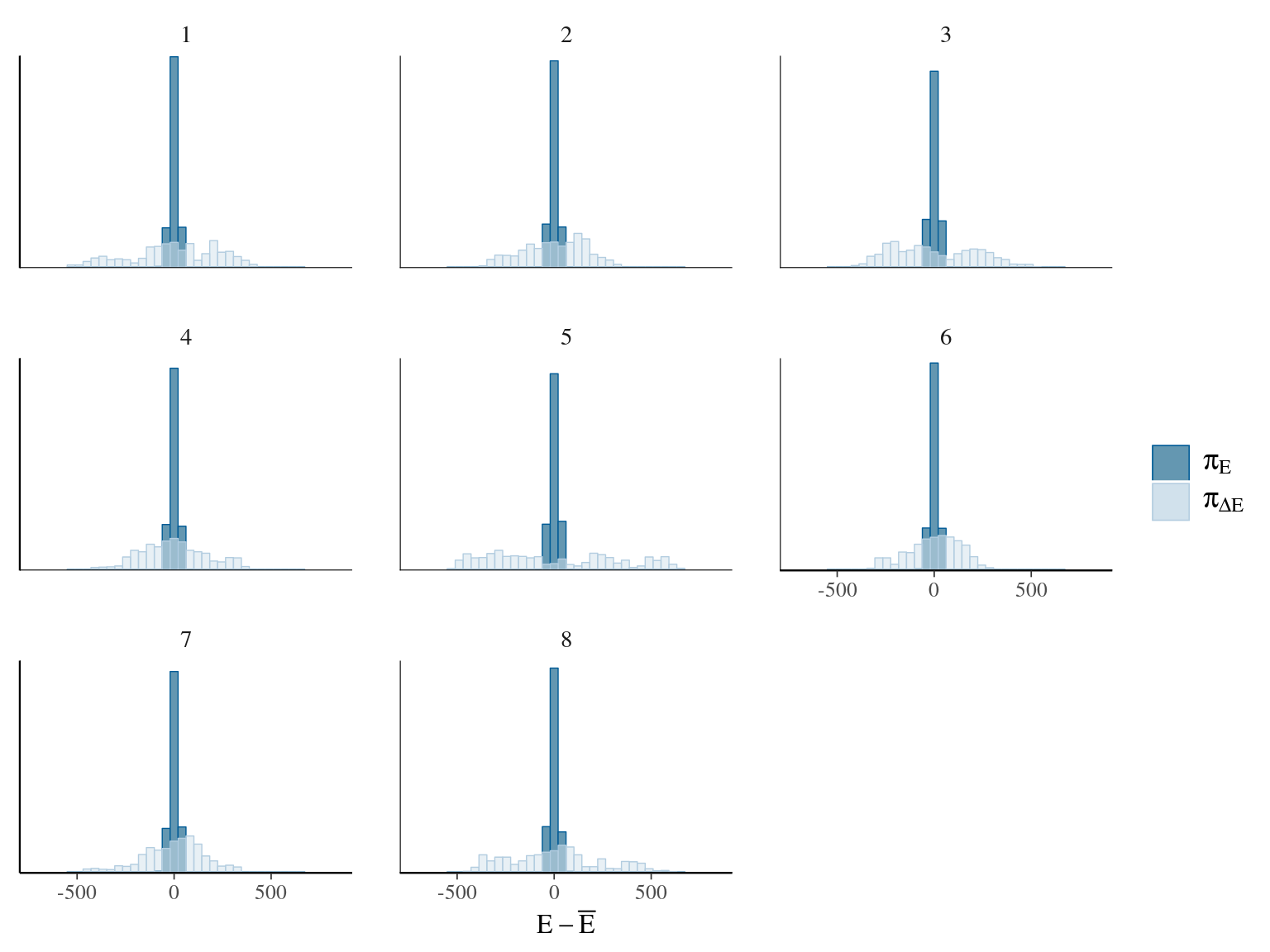
Figure 22.3: Energy of the model.

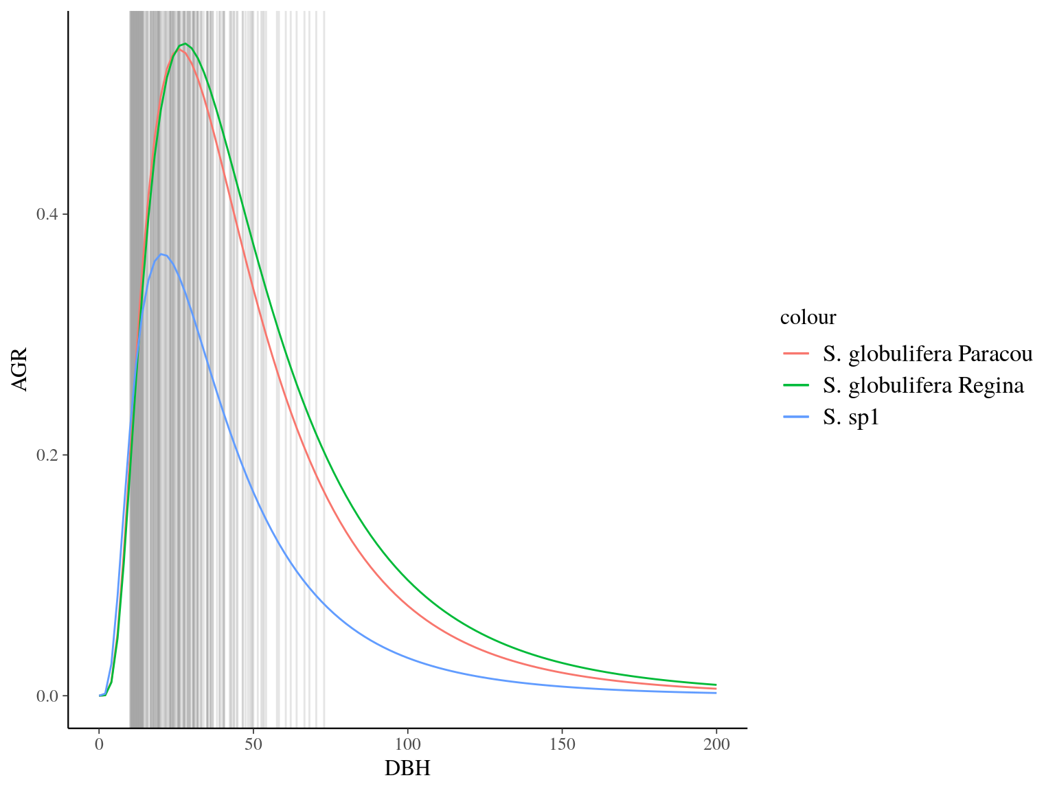
Figure 22.4: Species predicted growth curve.

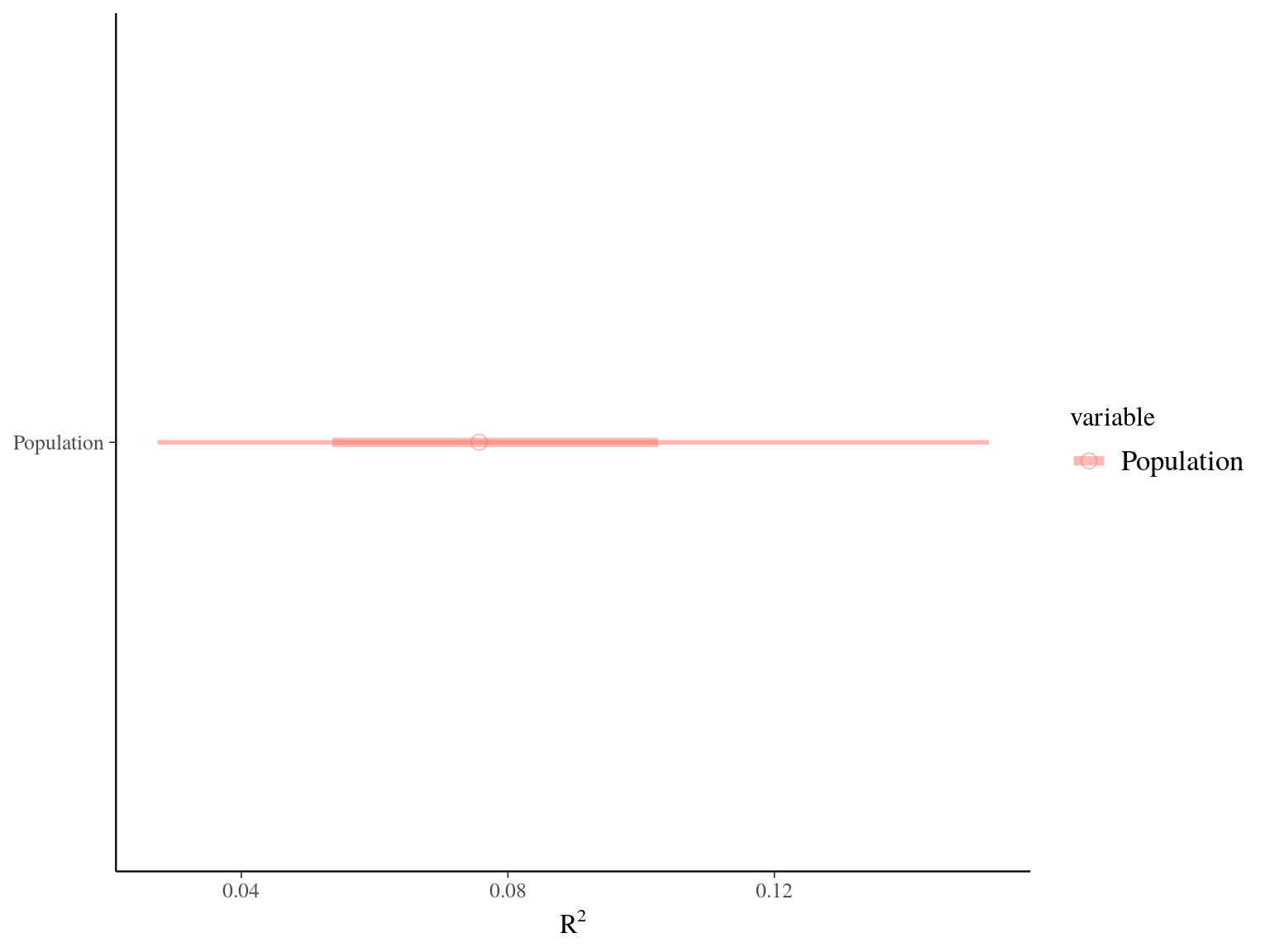
Figure 22.5: R2 for Gmax.

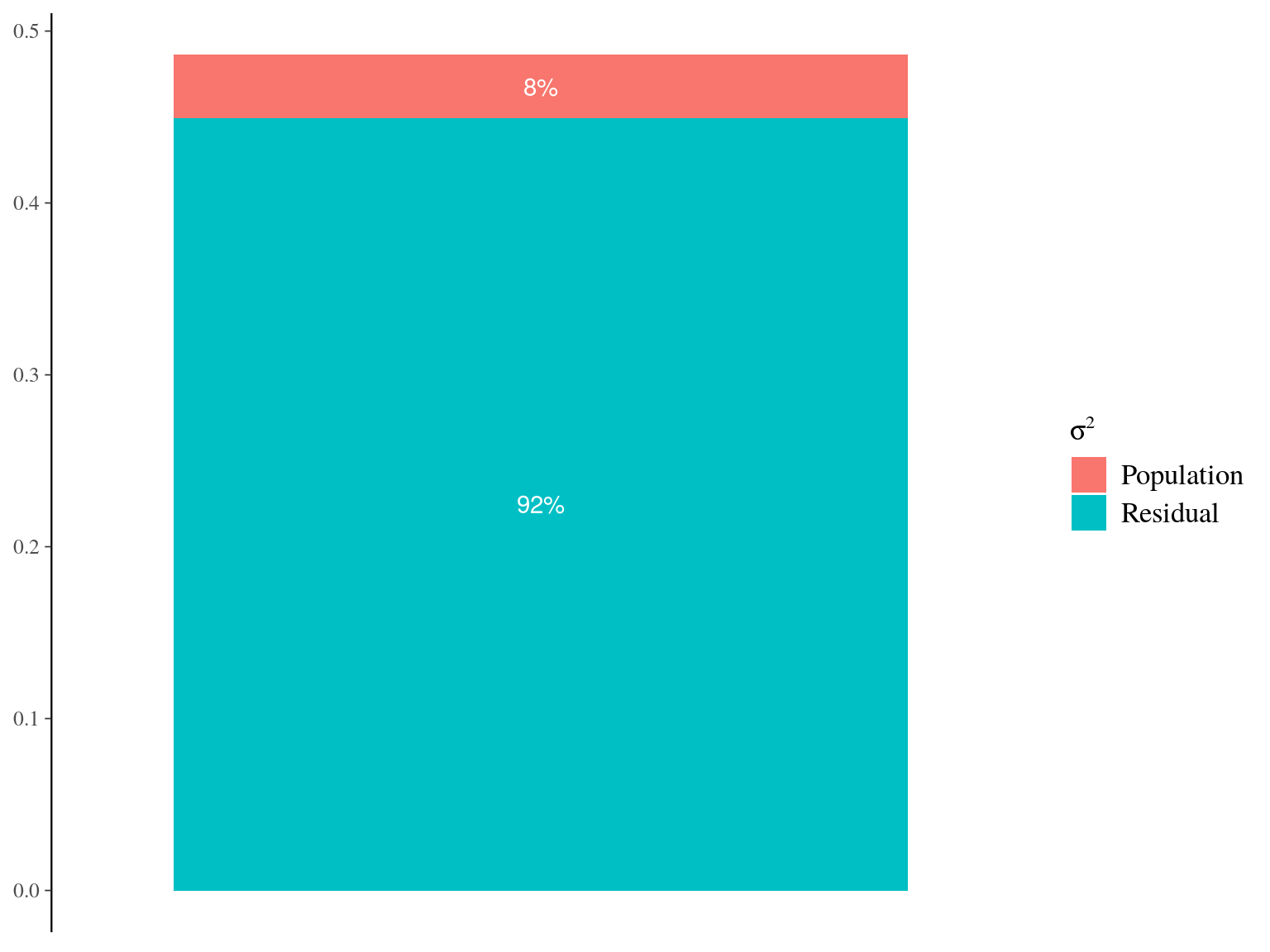
Figure 22.6: Genetic variance partitionning for Gmax.

22.2 Gmax & Genotype

We used the following growth model with a lognormal distribution to estimate individual growth potential and associated genotypic variation:

\[\begin{equation} DBH_{y=today,p,i} - DBH_{y=y0,p,i} \sim \\ \mathcal{logN} (log(\sum _{y=y_0} ^{y=today} \theta_{1,p,i}.exp(-\frac12.[\frac{log(\frac{DBH_{y,p,i}}{100.\theta_{2,p}})}{\theta_{3,p}}]^2)), \sigma_1) \\ \theta_{1,p,i} \sim \mathcal {logN}(log(\theta_{1,p}.a_{1,i}), \sigma_2) \\ \theta_{2,p} \sim \mathcal {logN}(log(\theta_2),\sigma_3) \\ \theta_{3,p} \sim \mathcal {logN}(log(\theta_3),\sigma_4) \\ a_{1,i} \sim \mathcal{MVlogN}(log(1), \sigma_5.K) \tag{22.3} \end{equation}\]

We fitted the equivalent model with following priors:

\[\begin{equation} DBH_{y=today,p,i} - DBH_{y=y0,p,i} \sim \\ \mathcal{logN} (log(\sum _{y=y_0} ^{y=today} \hat{\theta_{1,p,i}}.exp(-\frac12.[\frac{log(\frac{DBH_{y,p,i}}{100.\hat{\theta_{2,p}}})}{\hat{\theta_{3,p}}}]^2)), \sigma_1) \\ \hat{\theta_{1,p,i}} = e^{log(\theta_{1,p}.\hat{a_{1,i}}) + \sigma_2.\epsilon_{1,i}} \\ \hat{\theta_{2,p}} = e^{log(\theta_2) + \sigma_3.\epsilon_{2,p}} \\ \hat{\theta_{3,p}} = e^{log(\theta_3) + \sigma_4.\epsilon_{3,p}} \\ \hat{a_{1,i}} = e^{\sigma_5.A.\epsilon_{4,i}} \\ \epsilon_{1,i} \sim \mathcal{N}(0,1) \\ \epsilon_{2,p} \sim \mathcal{N}(0,1) \\ \epsilon_{3,p} \sim \mathcal{N}(0,1) \\ \epsilon_{4,i} \sim \mathcal{N}(0,1) \\ ~ \\ (\theta_{1,p}, \theta_2, \theta_3) \sim \mathcal{logN}^3(log(1),1) \\ (\sigma_1, \sigma_2, \sigma_3, \sigma_4, \sigma_5) \sim \mathcal{N}^5_T(0,1) \\ ~ \\ V_P = Var(log(\mu_p)) \\ V_G=\sigma_5^2\\ V_R=\sigma_2^2 \tag{22.4} \end{equation}\]

Table 22.2: Individual growth potential model.
Parameter	Estimate	Standard error	\(\hat R\)	\(N_{eff}\)
thetap1[1]	0.5427844	0.0705194	1.002621	1588
thetap1[2]	0.5593631	0.1088714	1.002237	1840
thetap1[3]	0.3484395	0.0303648	1.002741	954
theta2	0.2527690	0.0845444	1.005552	1944
theta3	0.6963378	0.1047527	1.007877	1064
sigma[1]	0.1487772	0.0727287	1.256714	33
sigma[2]	0.4964445	0.1739066	1.098502	57
sigma[3]	0.2800740	0.2970960	1.000608	2252
sigma[4]	0.1381212	0.2356811	1.003299	2446
sigma[5]	0.4759487	0.1820254	1.067011	69
lp__	138.6716378	192.6501649	1.379743	24

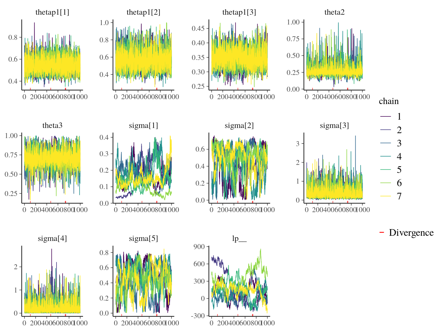
Figure 22.7: Traceplot of model parameters.

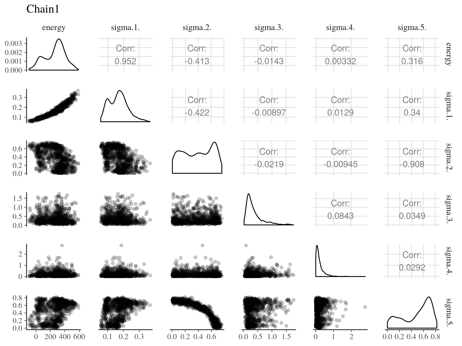
Figure 22.8: Pairs of model parameters.

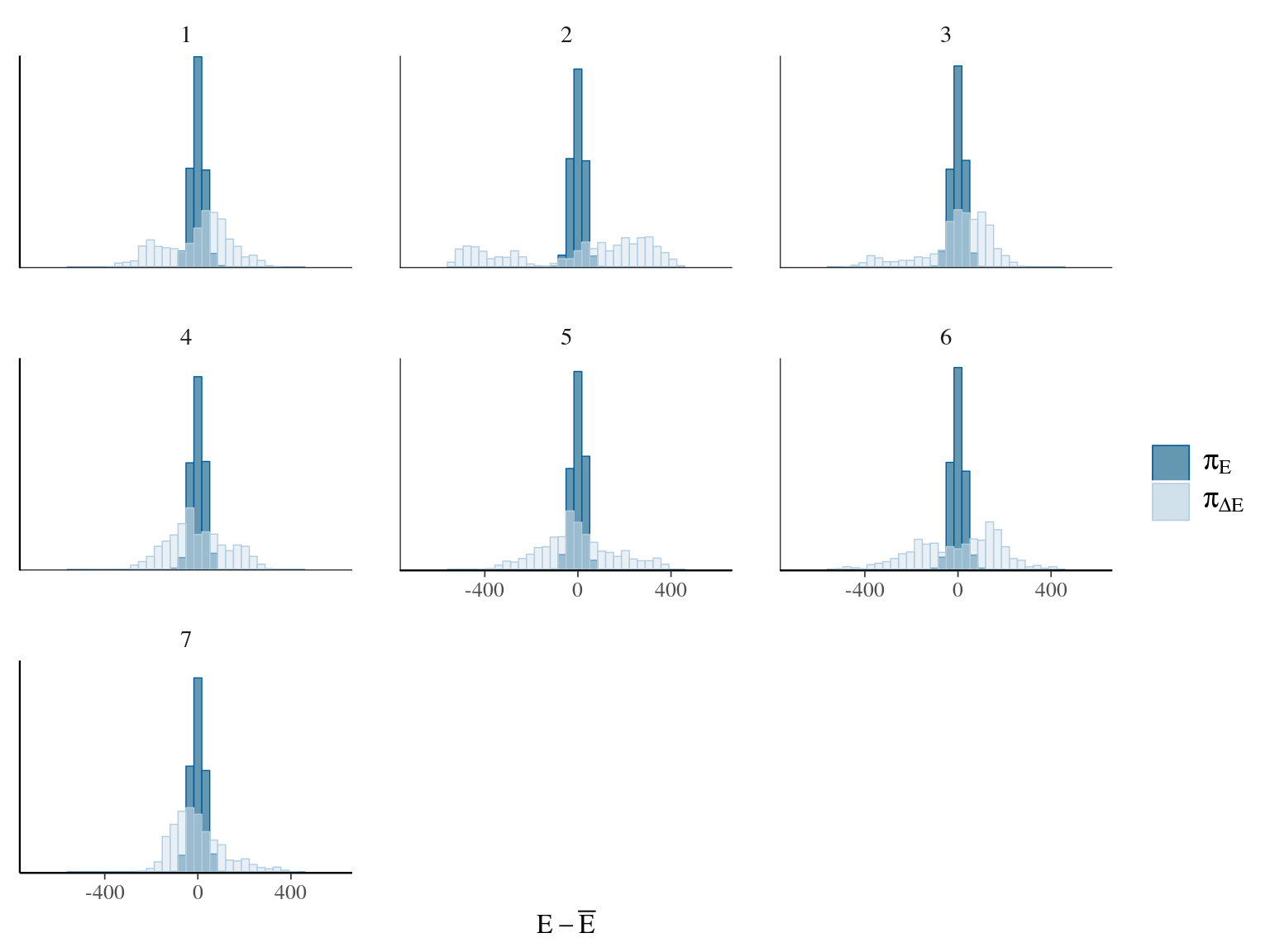
Figure 22.9: Energy of the model.

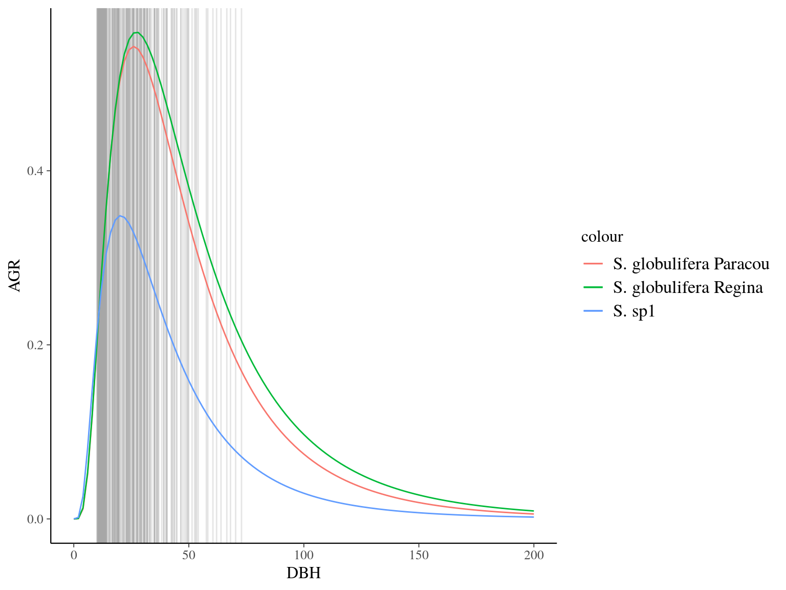
Figure 22.10: Species predicted growth curve.

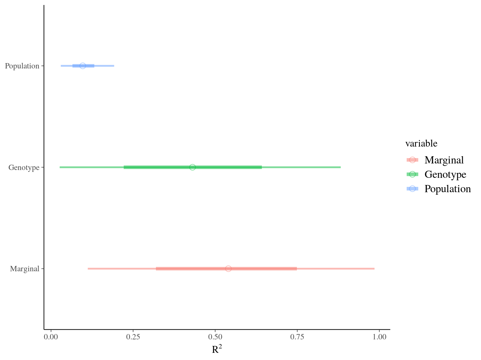
Figure 22.11: R2 for Gmax.

Figure 22.12: Genetic variance partitionning for Gmax.

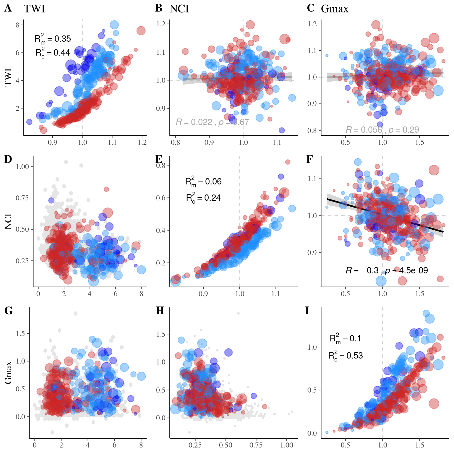
Figure 22.13: Long legend…

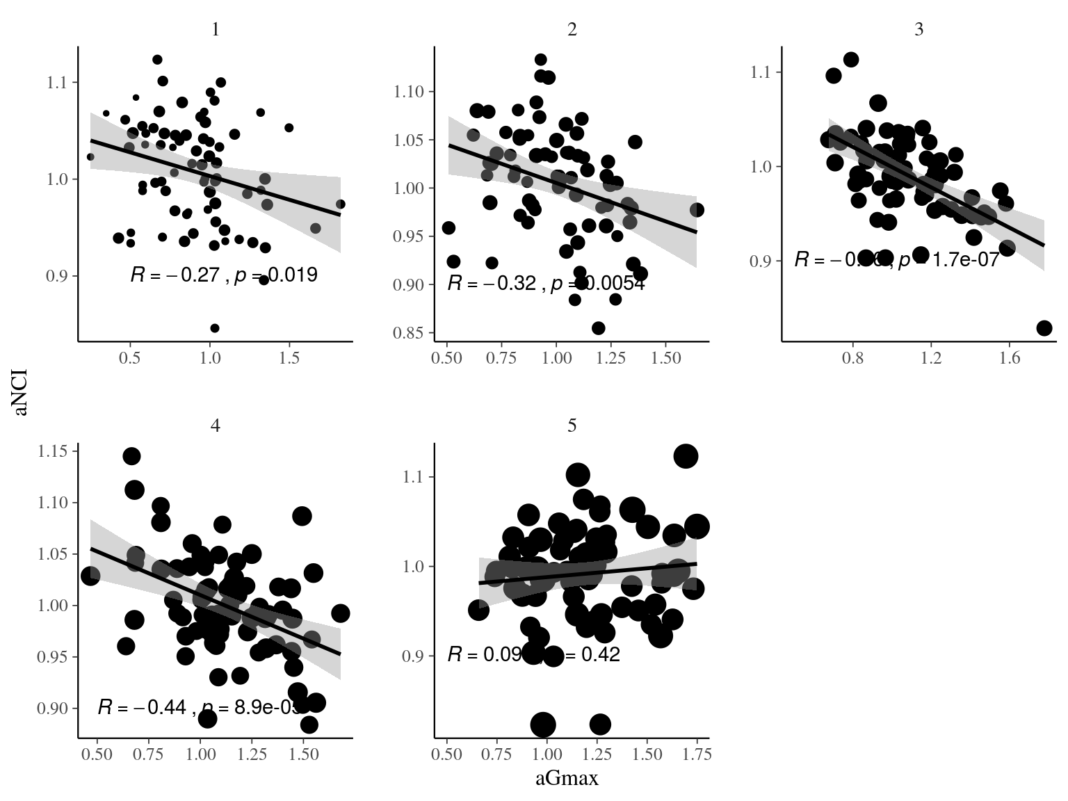
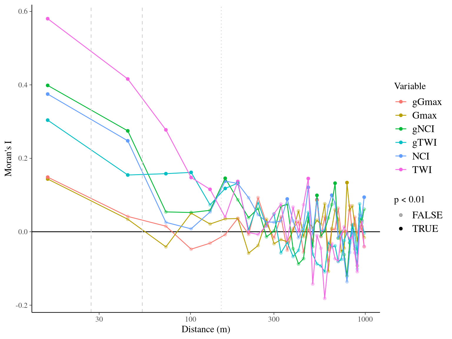
Figure 22.14: Spatial autocorrelogram (Moran’s I) of variables and associated genetic multiplicative values.

22.3 Gmax, Genotype & Environment

We used the following growth model with a lognormal distribution to estimate individual growth potential and associated genotypic variation:

\[\begin{equation} DBH_{y=today,p,i} - DBH_{y=y0,p,i} \sim \\ \mathcal{logN} (log(\sum _{y=y_0} ^{y=today} \theta_{1,p,i}.exp(-\frac12.[\frac{log(\frac{DBH_{y,p,i}}{100.\theta_{2,p}})}{\theta_{3,p}}]^2)), \sigma_1) \\ \theta_{1,p,i} \sim \mathcal {logN}(log(\theta_{1,p}.a_{1,i}. \beta_1.TWI_i.\beta_2.NCI_i), \sigma_2) \\ \theta_{2,p} \sim \mathcal {logN}(log(\theta_2),\sigma_3) \\ \theta_{3,p} \sim \mathcal {logN}(log(\theta_3),\sigma_4) \\ a_{1,i} \sim \mathcal{MVlogN}(log(1), \sigma_5.K) \tag{22.5} \end{equation}\]

We fitted the equivalent model with following priors:

\[\begin{equation} DBH_{y=today,p,i} - DBH_{y=y0,p,i} \sim \\ \mathcal{logN} (log(\sum _{y=y_0} ^{y=today} \hat{\theta_{1,p,i}}.exp(-\frac12.[\frac{log(\frac{DBH_{y,p,i}}{100.\hat{\theta_{2,p}}})}{\hat{\theta_{3,p}}}]^2)), \sigma_1) \\ \hat{\theta_{1,p,i}} = e^{log(\theta_{1,p}.\hat{a_{1,i}}. \beta_1.TWI_i.\beta_2.NCI_i) + \sigma_2.\epsilon_{1,i}} \\ \hat{\theta_{2,p}} = e^{log(\theta_2) + \sigma_3.\epsilon_{2,p}} \\ \hat{\theta_{3,p}} = e^{log(\theta_3) + \sigma_4.\epsilon_{3,p}} \\ \hat{a_{1,i}} = e^{\sigma_5.A.\epsilon_{4,i}} \\ \epsilon_{1,i} \sim \mathcal{N}(0,1) \\ \epsilon_{2,p} \sim \mathcal{N}(0,1) \\ \epsilon_{3,p} \sim \mathcal{N}(0,1) \\ \epsilon_{4,i} \sim \mathcal{N}(0,1) \\ ~ \\ (\theta_{1,p}, \theta_2, \theta_3) \sim \mathcal{logN}^3(log(1),1) \\ (\sigma_1, \sigma_2, \sigma_3, \sigma_4, \sigma_5) \sim \mathcal{N}^5_T(0,1) \\ ~ \\ V_P = Var(log(\mu_p)) \\ V_G=\sigma_5^2\\ V_{TWI} = Var(log(\beta_1.TWI_i)) \\ V_{NCI} = Var(log(\beta_2.NCI_i)) \\ V_R=\sigma_2^2 \tag{22.6} \end{equation}\]

Table 22.3: Individual growth potential model.
Parameter	Estimate	Standard error	\(\hat R\)	\(N_{eff}\)
thetap1[1]	0.6819703	0.1750196	1.0017710	3771
thetap1[2]	0.4693647	0.1630881	1.0003561	3238
thetap1[3]	0.7133448	0.1741461	1.0009126	3999
beta[1]	1.0338461	0.4773498	1.0009493	5751
beta[2]	1.0231845	0.4821474	0.9998852	6093
theta2	0.2212118	0.0872344	1.0031382	1564
theta3	0.6542952	0.1080025	1.0011451	2755
sigma[1]	0.1302832	0.0953805	1.3708842	22
sigma[2]	0.8841277	0.1185958	1.1145255	81
sigma[3]	0.3078621	0.3262250	1.0020929	2855
sigma[4]	0.1441136	0.2493211	1.0005756	4162
sigma[5]	0.4157660	0.2270843	1.1430011	55
lp__	184.4453908	241.4955933	1.6103979	13

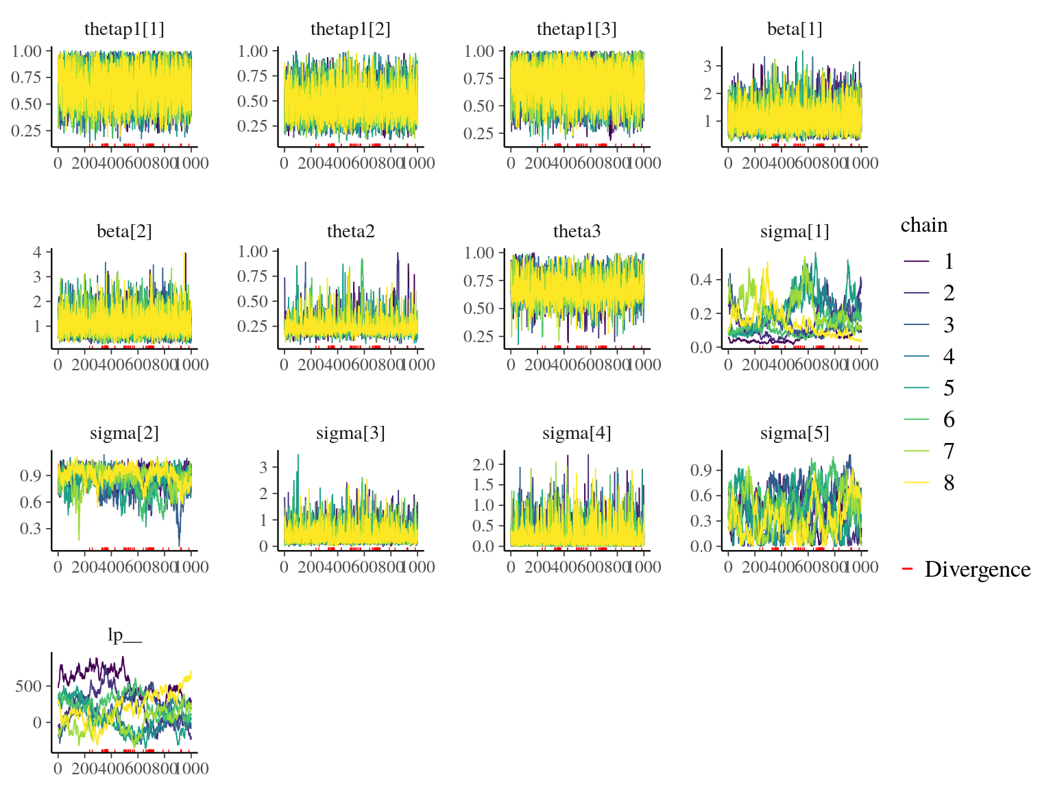
Figure 22.15: Traceplot of model parameters.

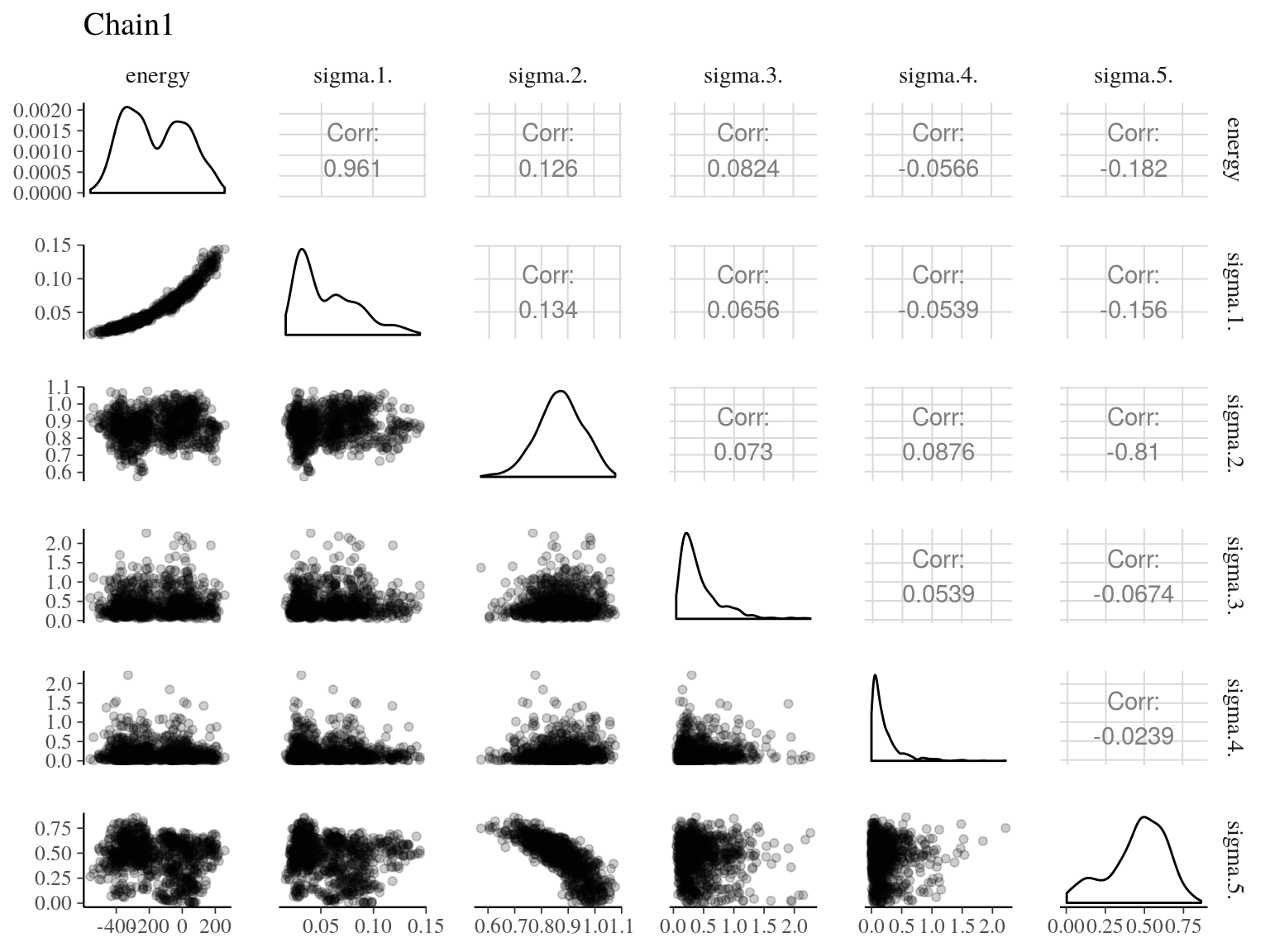
Figure 22.16: Pairs of model parameters.

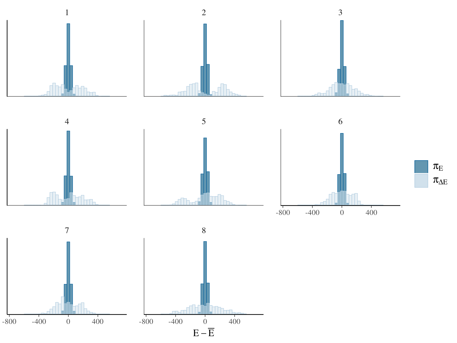
Figure 22.17: Energy of the model.

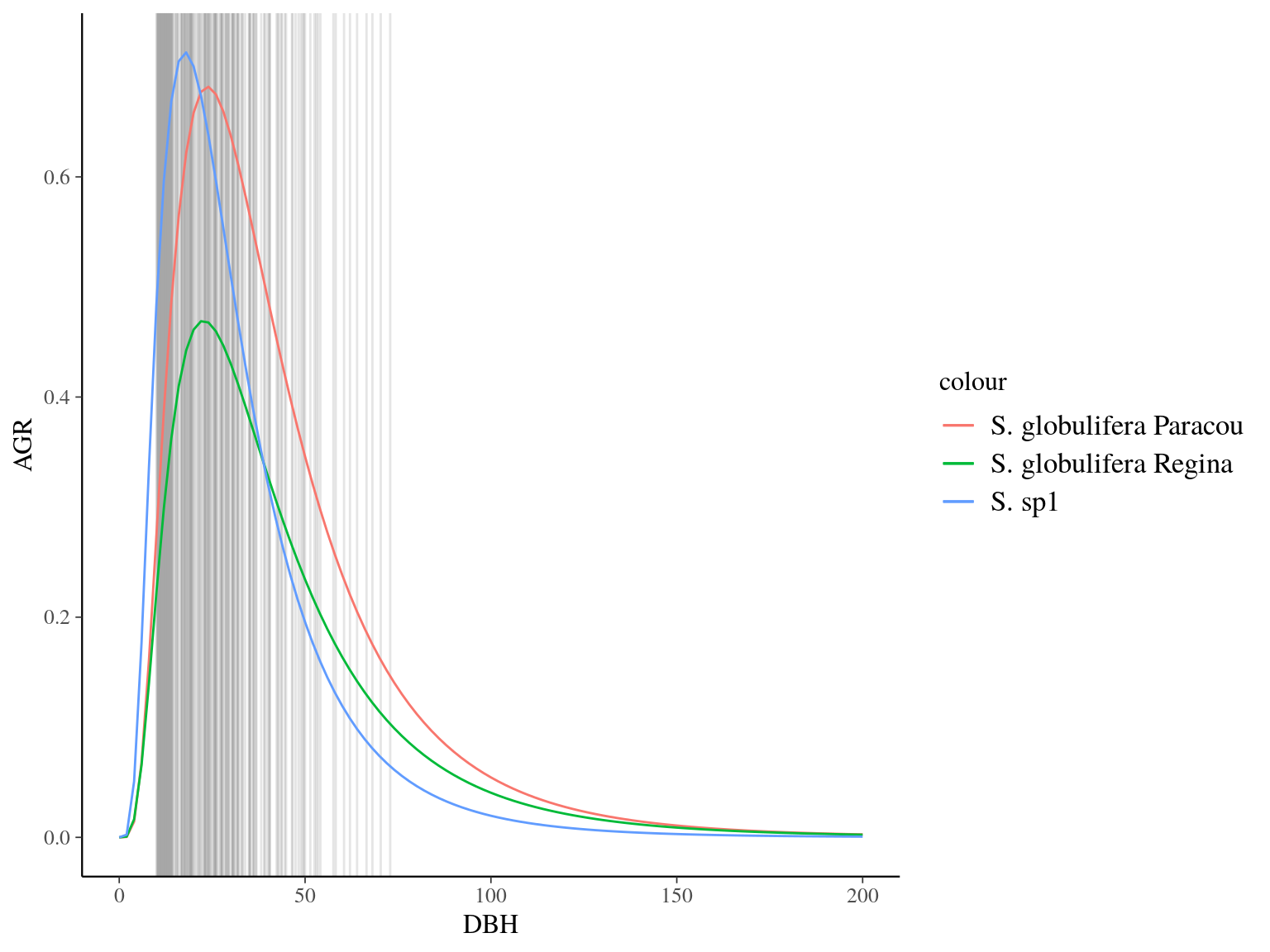
Figure 22.18: Species predicted growth curve.

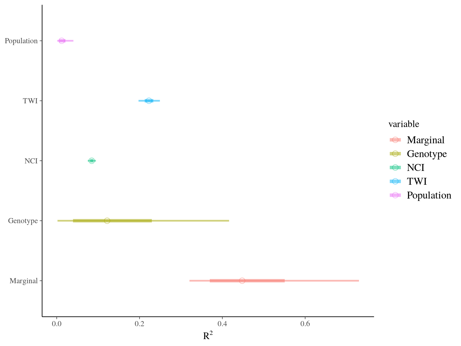
Figure 22.19: R2 for Gmax.

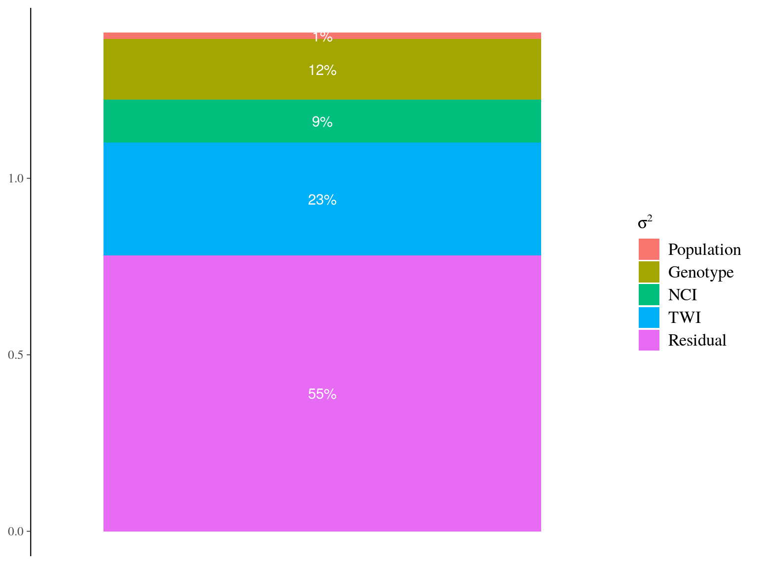
Figure 22.20: Genetic variance partitionning for ontogenetic parameters.

22.4 Associations

SNP association to growth potential \(Gmax\) has been assessed per individual with mono- and poly-genic modelling (respectivelly LMM and BSLMM, see methods in environmental genomics) for every populations.

module load bioinfo/plink-v1.90b5.3
module load bioinfo/gemma-v0.97
pops=(globuliferaTypeParacou globuliferaTypeRegina sp1)
for pop in "${pops[@]}" ; 
  do 
    plink \
      --bfile growth \
      --allow-extra-chr \
      --keep  $pop.fam \
      --extract growth.prune.in \
      --maf 0.05 \
      --pheno gmax.phenotype \
      --out $pop --make-bed ; 
    gemma -bfile $pop -gk 1 -o kinship.$pop ;
    gemma -bfile $pop -lmm 1 \
      -k output/kinship.$pop.cXX.txt \
      -o LMM.$pop ;
done
cat LMM.snps | cut -f1 > snps.list
plink --bfile growth --allow-extra-chr --extract snps.list --out outliers --recode A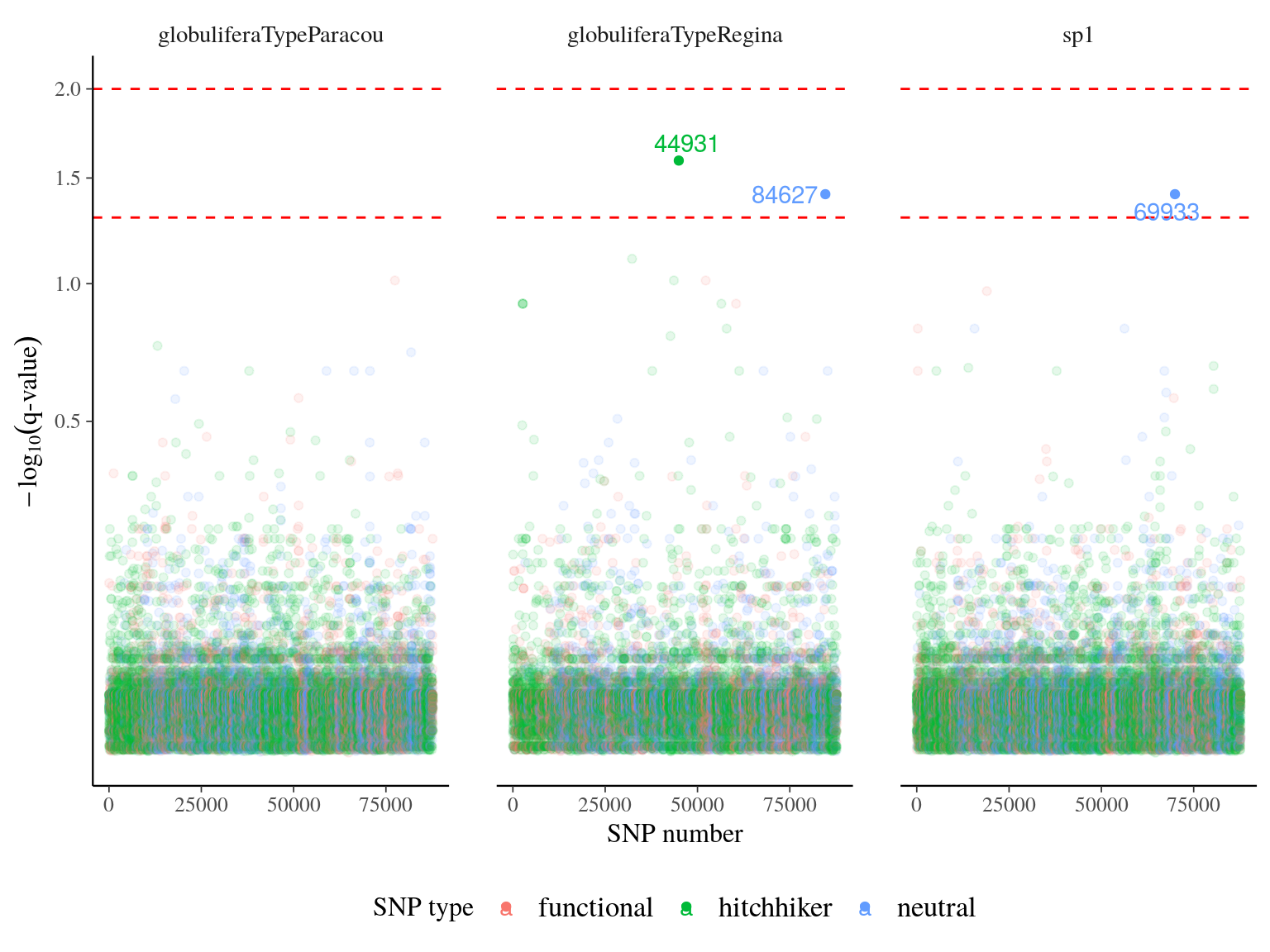

q-value of major effect SNPs associated to individual growth parameters. SNP were detected using linear mixed models (LMM) with individual kiniship as random effect. SNP significance was assessed with Wald test. q-value was obtained correcting mutlitple testing with false discovery rate.

Figure 22.21: q-value of major effect SNPs associated to individual growth parameters. SNP were detected using linear mixed models (LMM) with individual kiniship as random effect. SNP significance was assessed with Wald test. q-value was obtained correcting mutlitple testing with false discovery rate.

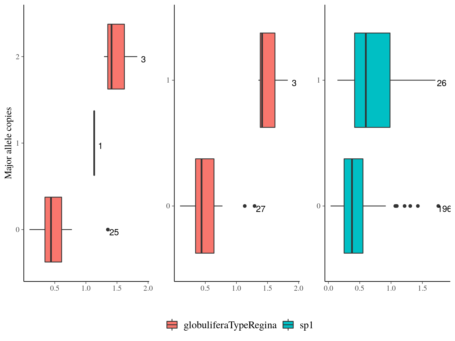
Figure 22.22: Growth parameters distribution for outliers genes.