Chapter 7 Plates
This chapter introduce the plates preparation after the extraction and before libraries preparation. First we will look into plates design after extraction. Then we will quantify their oncentration, volume and DNA quantity, before rearranging them based on their concentration. Finally plates concentration will be adjusted to 20 \(ng.\mu L^{-1}\) and sorted by electrophoresis evaluation.
7.1 Extraction
7.1.1 Extraction Plates
Plates after extraction were arranged following figure 7.1.
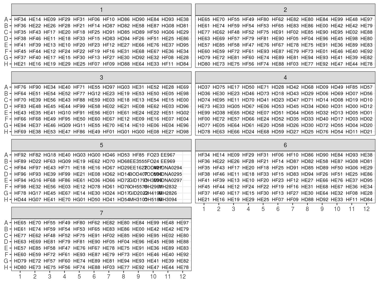
Figure 7.1: Extraction plates organization
All plates will be quantified through NanoDrop and some of them with Qbit which is more precise. We will use Qbit-NanoDrop relation to have an estimation of concentration for all samples. Finally electrophoresis are also used to asses DNA quality and degradation.
7.1.2 Extraction NanoDrop
NanoDrop evaluated \(1 \mu L\) of samples DNA concentration (figure 7.2) by absorption in addition to contamination. But NanoDrop is known to be inaccurate, especially under 25 \(ng.\mu L^{-1}\).
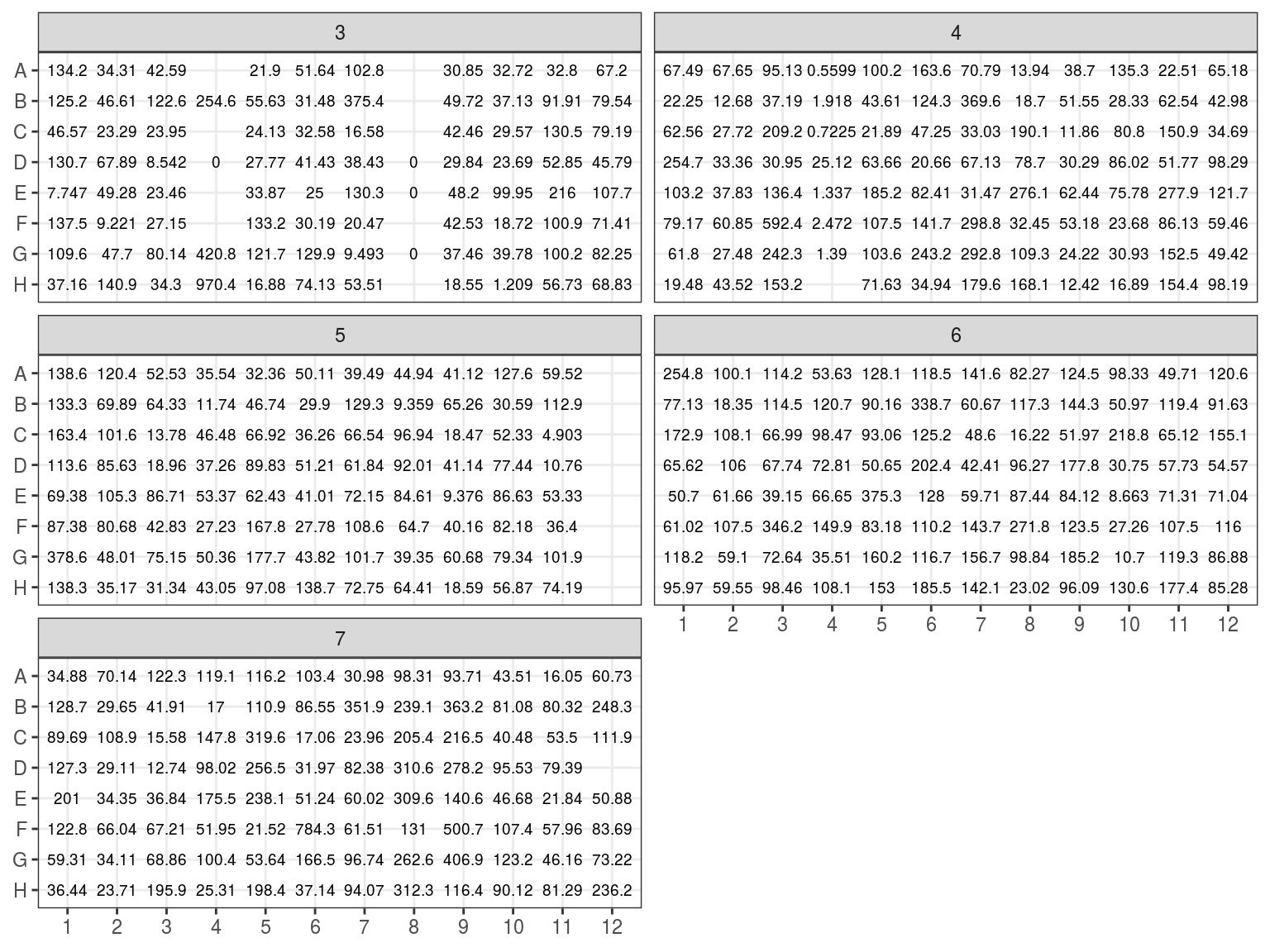
Figure 7.2: Extraction plate NanoDrop concentration (in ng/microL)
7.1.3 Extraction QBit
We used Qbit on 12 samples to have a more precise idea of samples concentration. Qbit is fluorescence to measure samples concentration in \(ng.\mu L^{-1}\). We compared QBit estimation of concentration to NanoDrop estimation. We used a bayesian approach to fit the model \(Concentration_{Qbit} \sim \mathcal{N}(\beta*Concentration_{NanoDrop},\sigma)\) with a null intercept. We found a pretty strong relation with a beta around 0.3. We thuse used this forumla to estimate better the concentration of all samples.
| term | estimate | std.error | rhat |
|---|---|---|---|
| beta | 0.2945394 | 0.0226193 | 0.9999254 |
| sigma | 8.3560063 | 2.2912140 | 1.0014413 |
| lp__ | -27.9855234 | 1.2573385 | 1.0044604 |
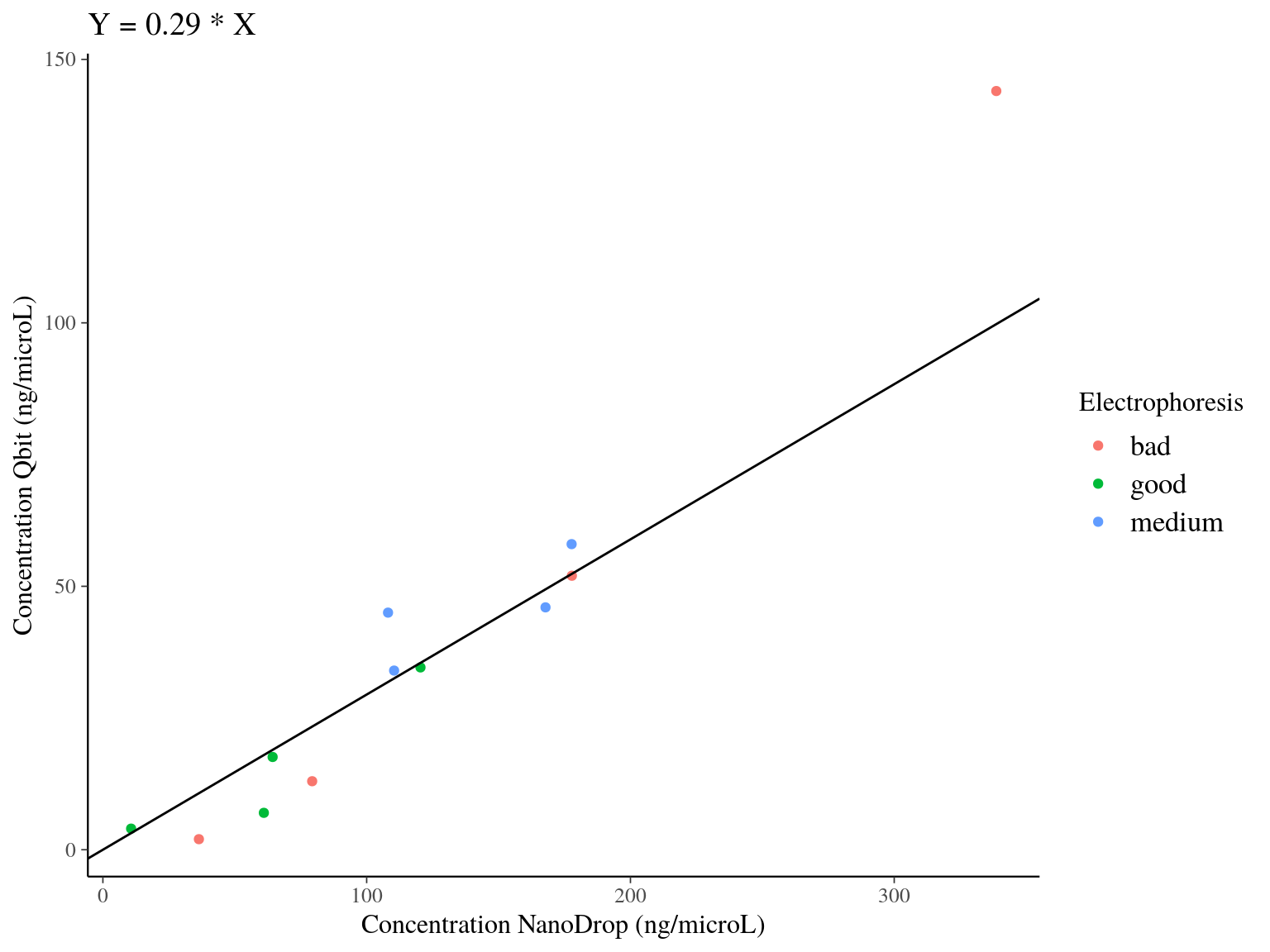
Figure 7.3: Model result of the relation between DNA concentration measured with Qbit and NanoDrop. Color indicates the electrophoresis classification of the samples.
7.1.4 Extraction Electrophoresis
We evaluated samples quality and degradation by an electrophoresis of 1 to 1.5 \(\mu L\) of sample DNA with 1 to 1.5 \(\mu L\) of weight migrating 20 minutes with 20 V on an agarose gel with 80 \(mL\) of 0.1 X TAE with 1 \(\mu L\) of red gel. Samples were classified as good, medium and bad. “Good” samples only included a band at high molecular weight, “bad” samples only included a smir at low molecular weight indicating degraded DNA, whereas “medium” samples included both.
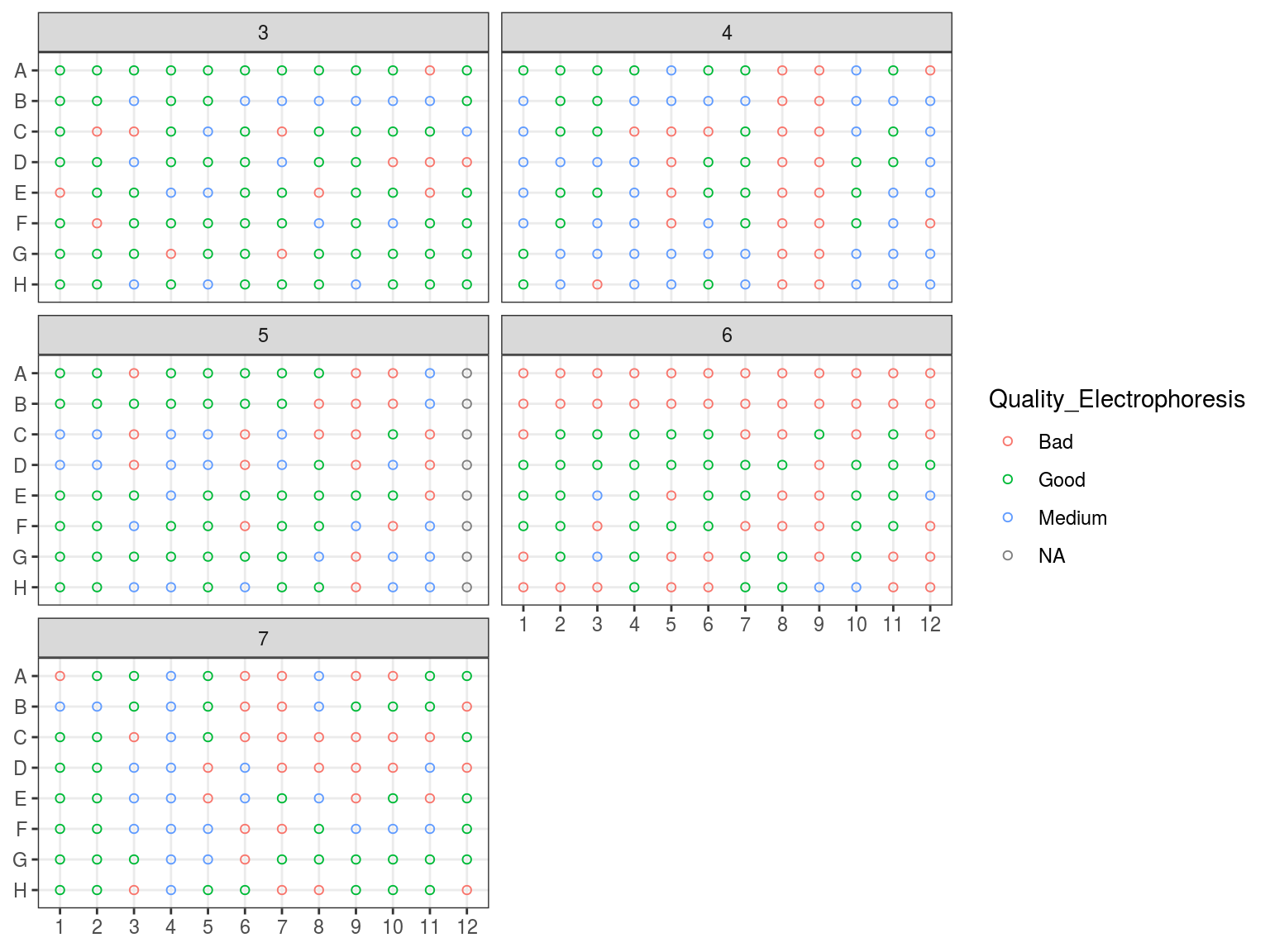
Figure 7.4: Extraction plate Electrophoresis quality
7.2 Library plates design
We first designed new plates based on the samples concentration in order to bring all samples to the same concentration for further easier manipulations in libraries preparation.
7.2.1 Pool
We pooled all individuals with 2 extraction and with a nanodrop concentration inferior to 25 \(ng.\mu L^{-1}\). Those wiht only one extraction will be further concentrated. Warning, P7-3-2812 has been pooled from P2.C12 to P7.C12 instead of P7.D12.
| ID | Plate_extraction | Position_extraction | nanodrop |
|---|---|---|---|
| P10_3_2912 | 1 | G10 | NA |
| P10_3_2912 | 6 | G10 | 10.70 |
| P11_1_742 | 3 | C2 | 23.29 |
| P11_1_742 | 5 | D3 | 18.96 |
| P13_2_2819 | 2 | F5 | NA |
| P13_2_2819 | 7 | F5 | 21.52 |
7.2.2 Pool and new samples nanodrop
Pooled individuals and new individuals from Itubera Brazil (n = 3), La Selva Costa Rica (n = 2) and Baro Colorado Island Panama (n = 2) has been quantified again with the nanodrop.
| ID | nanodrop | Plate | Position |
|---|---|---|---|
| P4-2-3487 | 20.71 | Pull | NA |
| LS-SG18 | 49.53 | America | NA |
| IT_H5 | 12.86 | Itubera | H5 |
| IT_H3 | 16.37 | Itubera | H3 |
| IT_B4 | 19.42 | Itubera | B4 |
7.2.3 Concentration Plates
We reorganised plates in a new scheme ordered by concentration followinf figure 7.5 design with figure 7.6 concentrations.
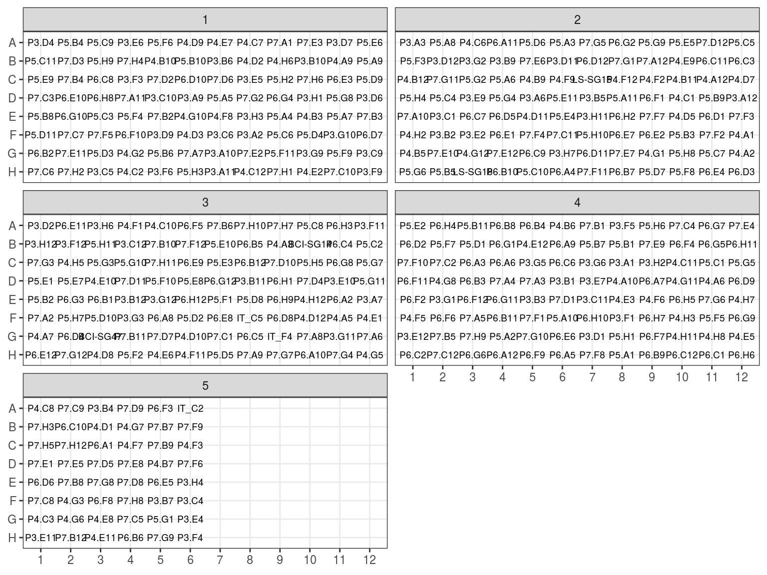
Figure 7.5: Previous extraction position in plates arranged by concentration.
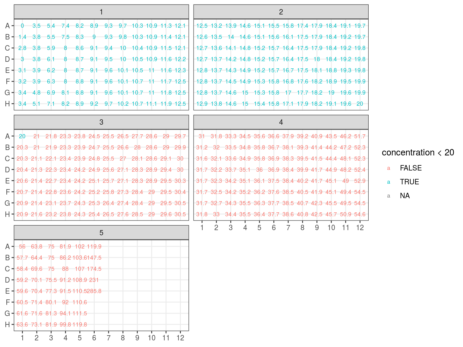
Figure 7.6: Concentration in plates arranged by concentration.
7.2.4 Samples volume
In order to adjust samples concentration we need first to assess their current volume, see figure 7.7. Volume after extraction was around 45 \(\mu L\) (estimated loss). Samples have lost volume with NanoDrop, Qbit, electrophoresis, and libraries trial, one or two times. And some sample won volume with pooling. We can consider all samples to have lost 1 \(\mu L\) with NanoDrop. Samples used in Qbit lost an additional 1.5 to 3 \(\mu L\). Finally samples used in trial libraries lost between 0.5 and 5 \(\mu L\) (with library test II repeated). And pooled samples from plate 5, 6 an 7 won 49 \(\mu L\) from NanoDroped samples from plate 1, 2, 3 and 4 unused for NanoDrop, Qbit nor libraries trial (original 50 minus 1 nanodropped). Added samples from Itubera, La Selva and Baro Colorado Island have an estimated volume of 10 \(\mu L\) (overestimated).
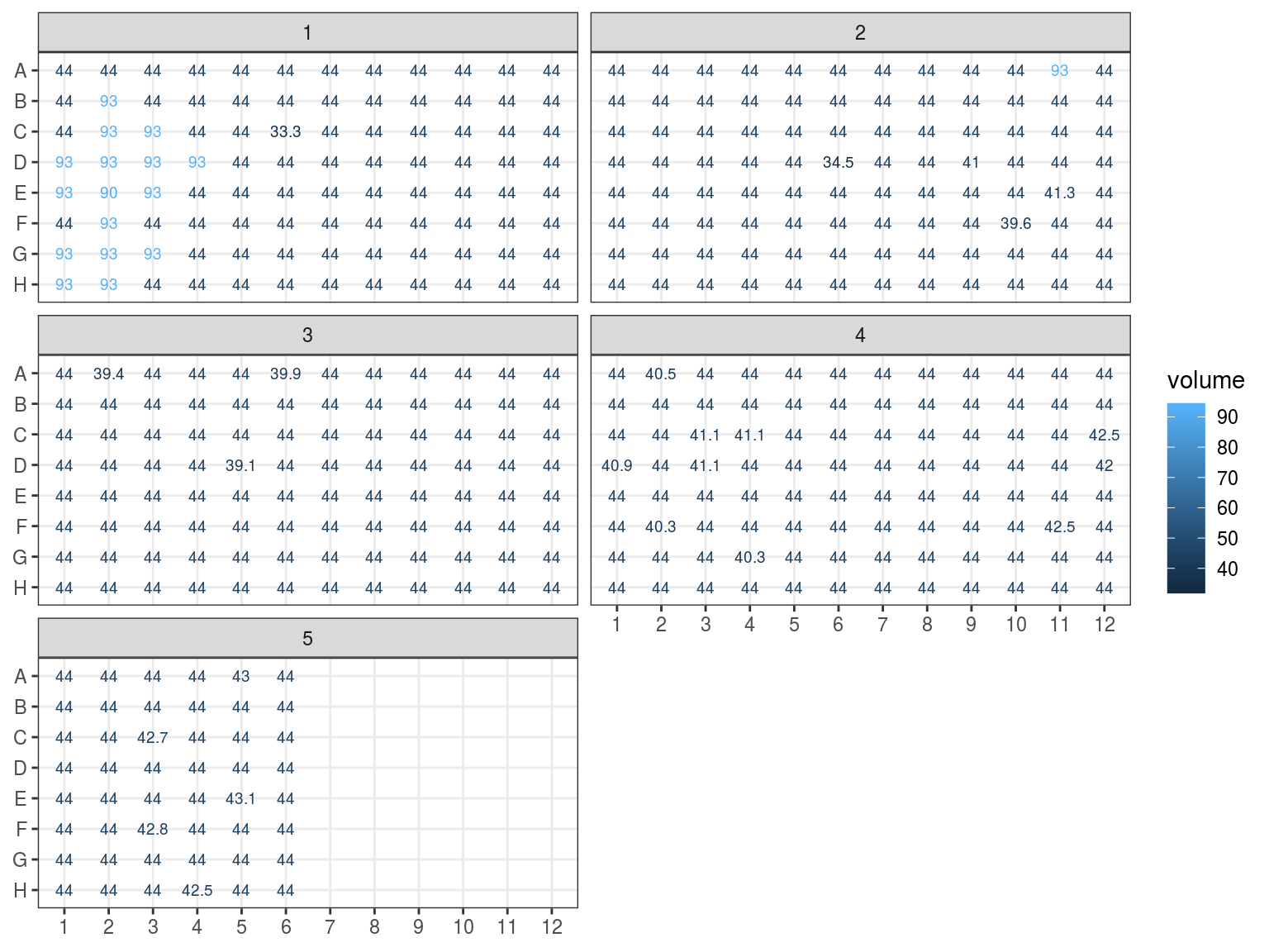
Figure 7.7: Samples estimated volumes.
7.2.5 DNA quality
We assessed DNA fragment quality and size through electrophoresis and reorganised columns inside plates by quality.
| ID | Plate_concentration | Position_concentration | volumeplus5 | concentration | Plate_library | Position_library |
|---|---|---|---|---|---|---|
| P15_3_267 | 1 | D1 | 98 | 3.004302 | 1 | B1 |
| P3_2_739 | 1 | E1 | 98 | 3.098555 | 1 | C1 |
| P5_4_658 | 1 | G1 | 98 | 3.357749 | 1 | E1 |
| P13_2_929 | 1 | H1 | 98 | 3.449056 | 1 | F1 |
| P13_4_149 | 1 | F2 | 98 | 3.932101 | 1 | G1 |
| P7_3_2837 | 1 | G2 | 98 | 4.765647 | 1 | H1 |
| P4_1_3000 | 1 | C3 | 98 | 5.899624 | 1 | C2 |
| P6_3_346 | 1 | E3 | 98 | 6.176491 | 1 | D2 |
| P11_1_742 | 1 | G3 | 98 | 6.912840 | 1 | E2 |
| P7_3_679 | 1 | B2 | 98 | 3.764213 | 1 | B4 |
| P15_4_40 | 1 | C2 | 98 | 3.831958 | 1 | C4 |
| P7_2_3049 | 1 | D2 | 98 | 3.849630 | 1 | F7 |
| P10_3_2912 | 1 | E2 | 95 | 3.914429 | 1 | G7 |
| P7_2_2520 | 1 | H2 | 98 | 5.089641 | 1 | H7 |
| P4_2_3487 | 1 | D3 | 98 | 6.099911 | 1 | A8 |
| P6_3_2800 | 1 | D4 | 98 | 8.002635 | 1 | D8 |
| P7_3_2812 | 2 | A11 | 98 | 19.130334 | 2 | F3 |
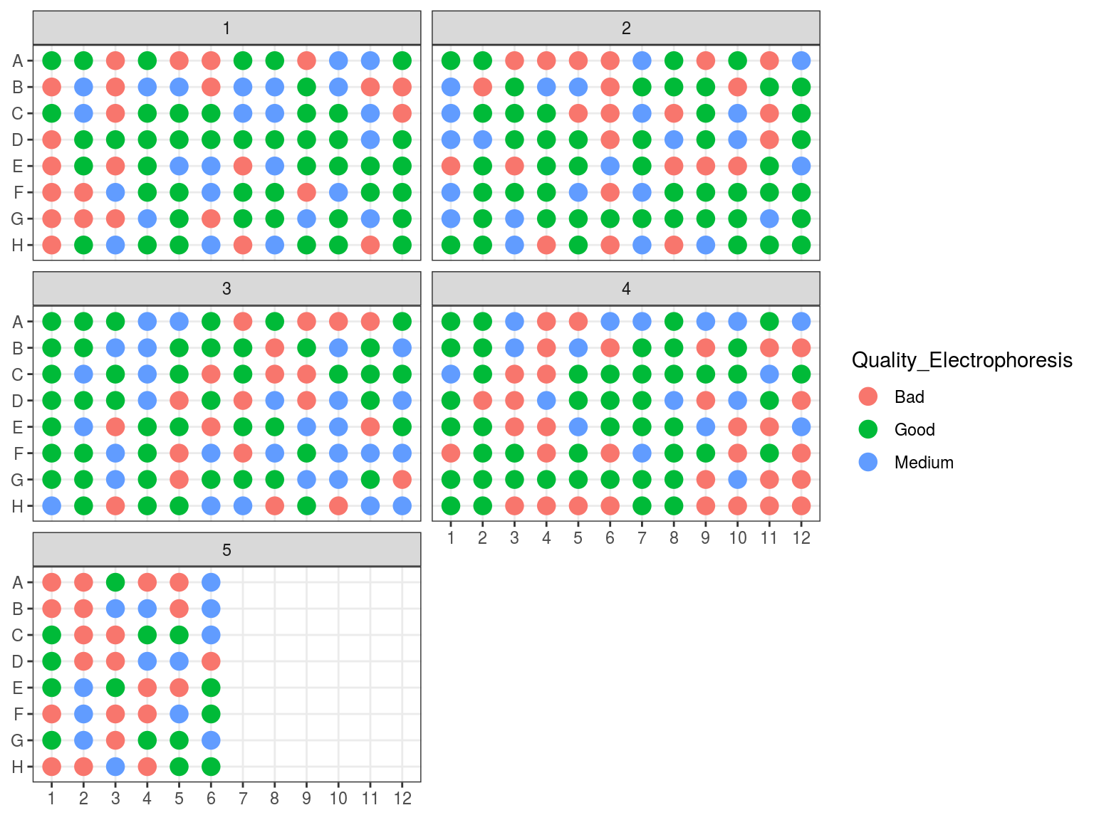
Figure 7.8: Plates electrophoresis status before rearrangement.
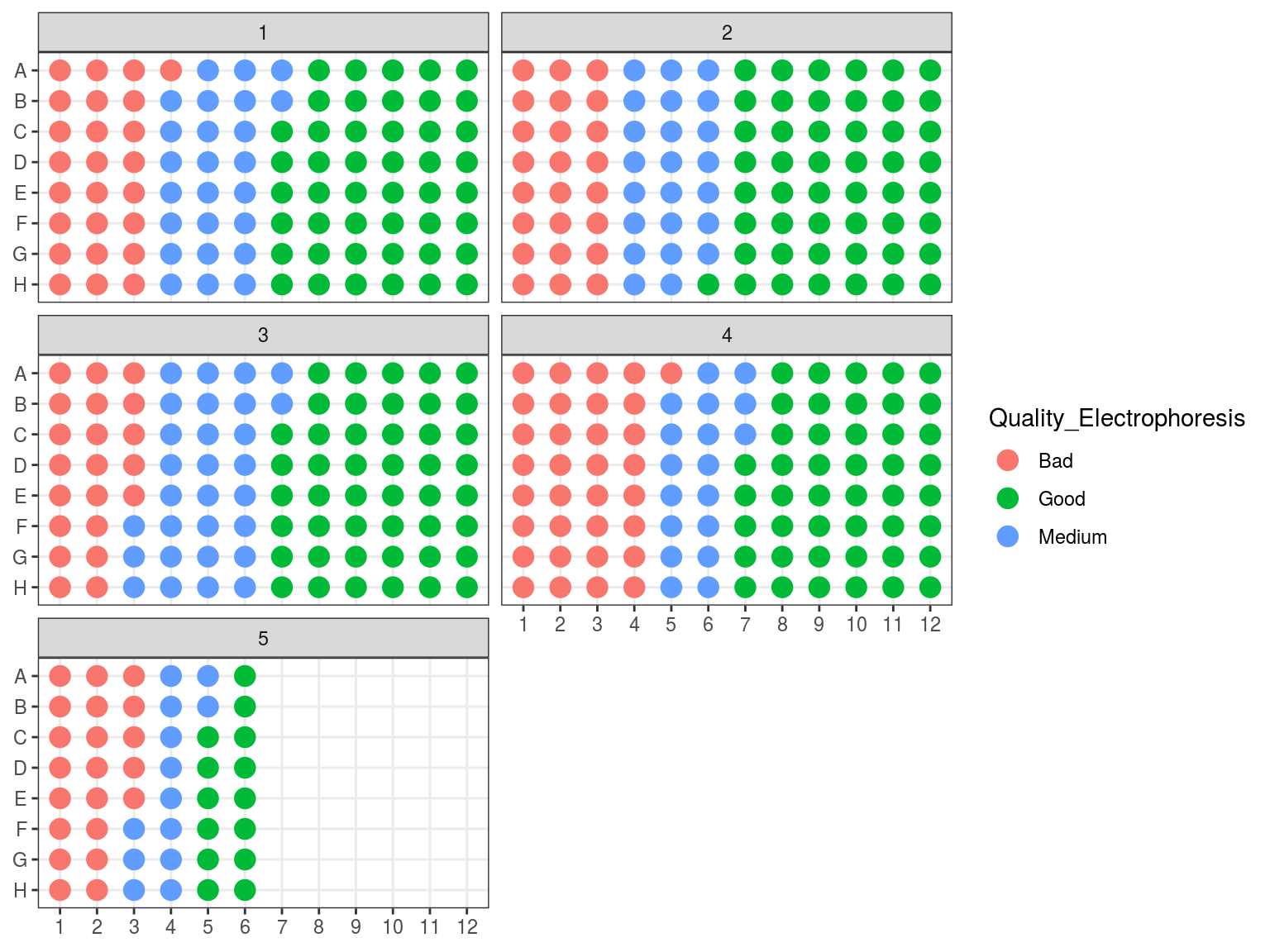
Figure 7.9: Plates electrophoresis status after rearrangement.
7.2.6 Concentration
All individuals with an estimated concetration inferior to 19 \(ng.\mu L^{-1}\) (Plates 1 and 2) have been dried in the speed vacuum centrifuge. And corresponding volume of miliQ water will be added to reach a concentration of 20 \(ng.\mu L^{-1}\) (or at least 6.5 \(\mu L\) to reach sample volume). Their DNA content in \(ng\) has beeen computed multiplying concentration with volume. The volume of water to add is thus the DNA content divided by the objective concentration of 20 \(ng.\mu L^{-1}\): \(V = \frac{C_0*V_0}{20}\). Corresponding volumes are shown in figure 7.11.
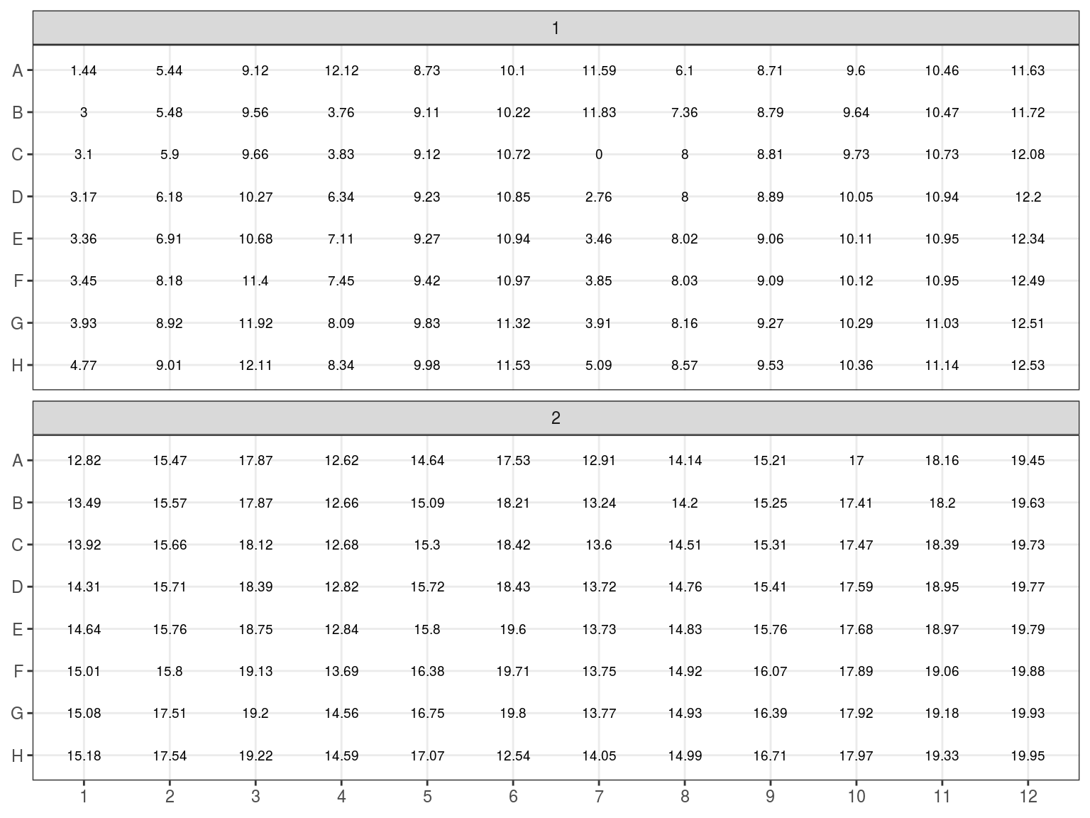
Figure 7.10: Samples to be concentrated. Estimated concentration in ng/microL
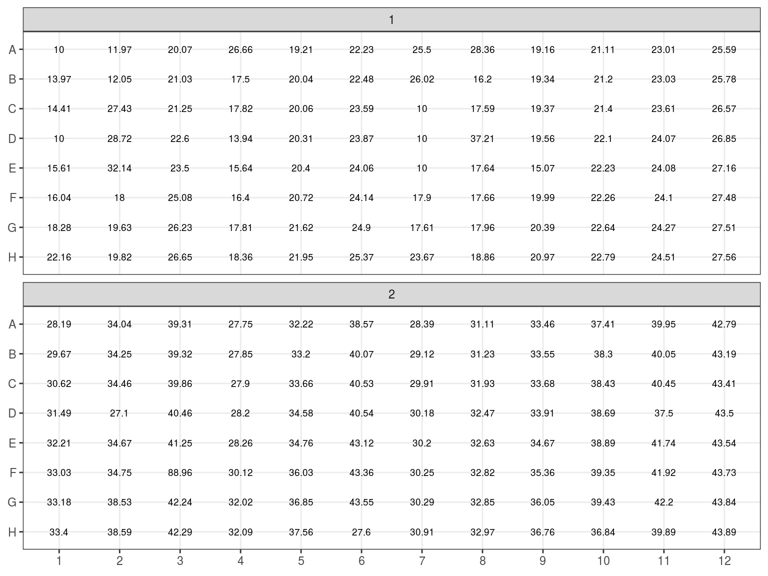
Figure 7.11: Volume to resupspend dry samples.
7.2.7 Samples volume
The objective is to get 100 \(ng\) of DNA in 6.5 \(\mu L\) of sample for the library preparation. Consequently we need to extract with the robot \(V = \frac{n}{C} = \frac{100}{C}\) with \(C\) the sample concentration in \(ng.\mu L^{-1}\).
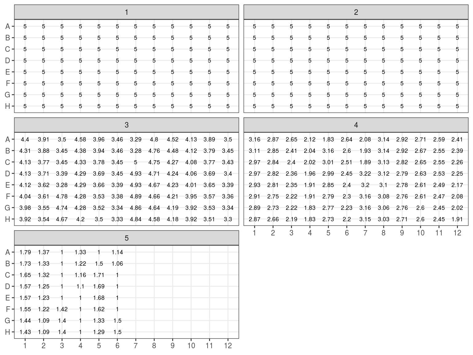
Figure 7.12: Sample volume (microL)
| Plate_library | Position_library | sample_volume | water_volume |
|---|---|---|---|
| 3 | F3 | 4.779183 | 1.720817 |
| 3 | G3 | 4.739818 | 1.760182 |
| 3 | H3 | 4.673915 | 1.826085 |
| 3 | A4 | 4.576266 | 1.923734 |
| 3 | C7 | 5.000930 | 1.499070 |
| 3 | D7 | 4.932633 | 1.567367 |
| 3 | E7 | 4.930484 | 1.569516 |
| 3 | F7 | 4.893531 | 1.606469 |
| 3 | G7 | 4.857822 | 1.642178 |
| 3 | H7 | 4.840507 | 1.659493 |
| 3 | A8 | 4.796061 | 1.703939 |
| 3 | B8 | 4.761088 | 1.738912 |
| 3 | C8 | 4.754420 | 1.745580 |
| 3 | D8 | 4.705657 | 1.794343 |
| 3 | E8 | 4.666848 | 1.833152 |
| 3 | F8 | 4.663002 | 1.836998 |
| 3 | G8 | 4.636891 | 1.863109 |
| 3 | H8 | 4.579970 | 1.920030 |
| 3 | A9 | 4.517806 | 1.982193 |