Chapter 15 Population structure
We explored population structure of individuals. Then, we quickly looked at th spatial and environmental distribution of the different gene pools and individual mismatch (before association genomic analyses).
- Structure population structure of all Symphonia individuals from Paracou with
admixture - Spatial spatial distribution of Symphonia gene pools in Paracou
- Mismatch spatial distribution of Symphonia gene pools in Paracou
- Environmental environmental distribution of Symphonia gene pools in Paracou along the topgraphic wetness index
- Kinship individuals kinship
15.1 Structure
Symphonia individuals are globally structured in three gene pools in Paracou corresponding to field morphotypes (Fig. 15.1 and Fig. 15.2). The three genotypes correspond to the previously identified two morphotypes (70-80%) S. globulifera and S. sp1, with S. globulifera morphotype structured in two gene pools, which might match the two identified submorphotype in Paracou called S. globulifera type Paracou (80%) and S. globulifera type Régina (20%). Interstingly, we noticed so-called Paracou type and Régina type within S. globulifera morphotype when sampling the individuals. And looking to few identified individuals bark, it seems that the two identified gene pools correspond two this two morphotypes (Fig. 15.5). The Paracou type have a smoother and thinner bark compared to the thck and lashed bark of Régina type.
module load bioinfo/admixture_linux-1.3.0
module load bioinfo/plink-v1.90b5.3
mkdir admixture
mkdir admixture/paracou
mkdir out
cd ../variantCalling
mkdir paracouRenamed
# read_tsv(file.path(pathCluster, "paracou", "symcapture.all.biallelic.snp.filtered.nonmissing.paracou.bim"),
#          col_names = F) %>%
#   mutate(X1 = as.numeric(as.factor(X1))) %>%
#   write_tsv(file.path(pathCluster, "paracouRenamed", "symcapture.all.biallelic.snp.filtered.nonmissing.paracou.bim"),
#             col_names = F)
cp paracou/symcapture.all.biallelic.snp.filtered.nonmissing.paracou.bed paracouRenamed
cp paracou/symcapture.all.biallelic.snp.filtered.nonmissing.paracou.fam paracouRenamed
cd ../populationGenomics/admixture/paracou
for k in $(seq 10) ; do echo "module load bioinfo/admixture_linux-1.3.0 ; admixture --cv ../../variantCalling/paracouRenamed/symcapture.all.biallelic.snp.filtered.nonmissing.paracou.bed $k | tee log$k.out" ; done > admixture.sh
sarray -J admixture -o ../../out/%j.admixture.out -e ../../out/%j.admixture.err -t 48:00:00 --mem=8G --mail-type=BEGIN,END,FAIL admixture.sh
scp sschmitt@genologin.toulouse.inra.fr:~/Symcapture/populationGenomics/admixture/paracou/*
grep -h CV log*.out > CV.out
for file in $(ls log*.out) ; do  grep "Fst divergences between estimated populations:" -A 20 $file | head -n -2 > matrices/$file ; done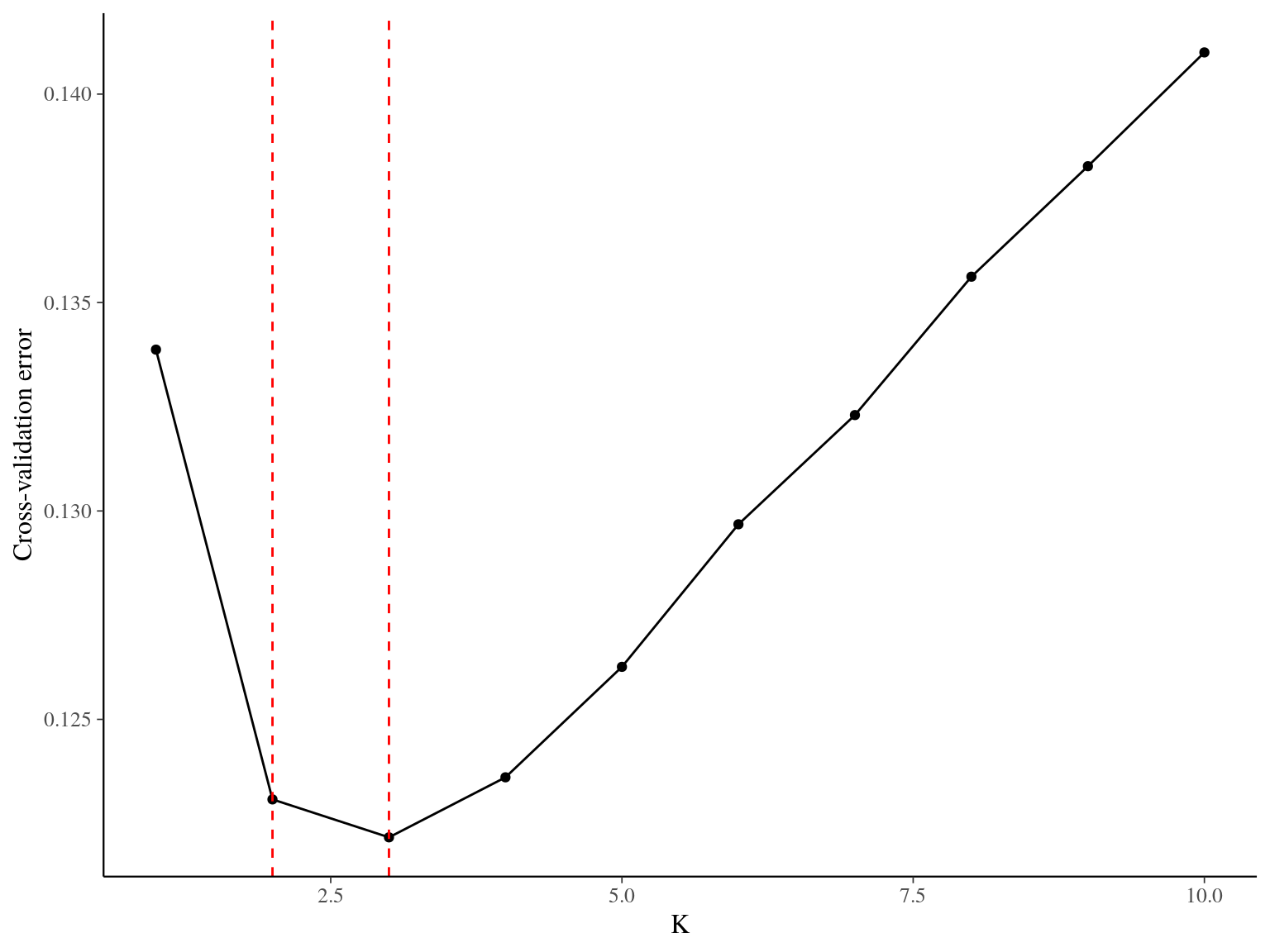
Figure 15.1: Cross-validation for the clustering of Paracou individuals. Y axis indicates corss-validation mean error, suggesting that 2 or 3 groups represent the best Paracou individuals structure.
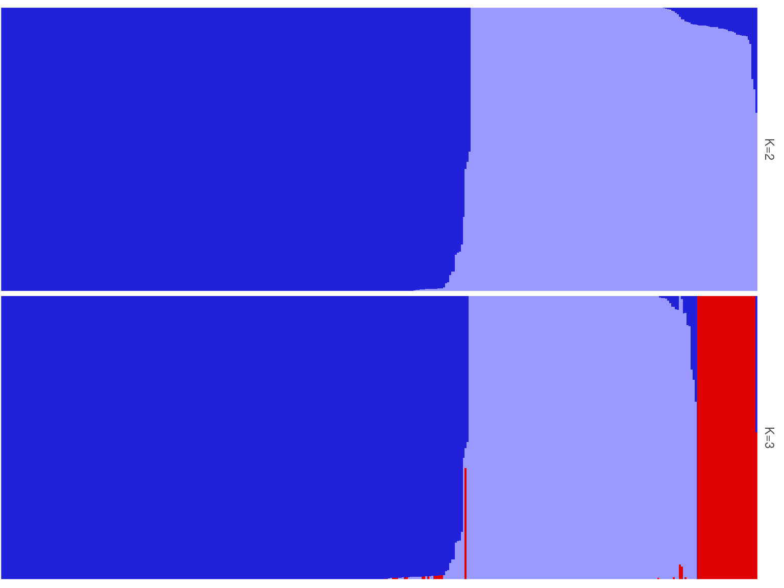
Figure 15.2: Population structure of Paracou individuals for K=2 and K=3. Dark blue is associated to S. globulifera morphotype; whereas light blue is associated to S. sp1; and red is associated to a subgroup within S. globulifera morphotype.
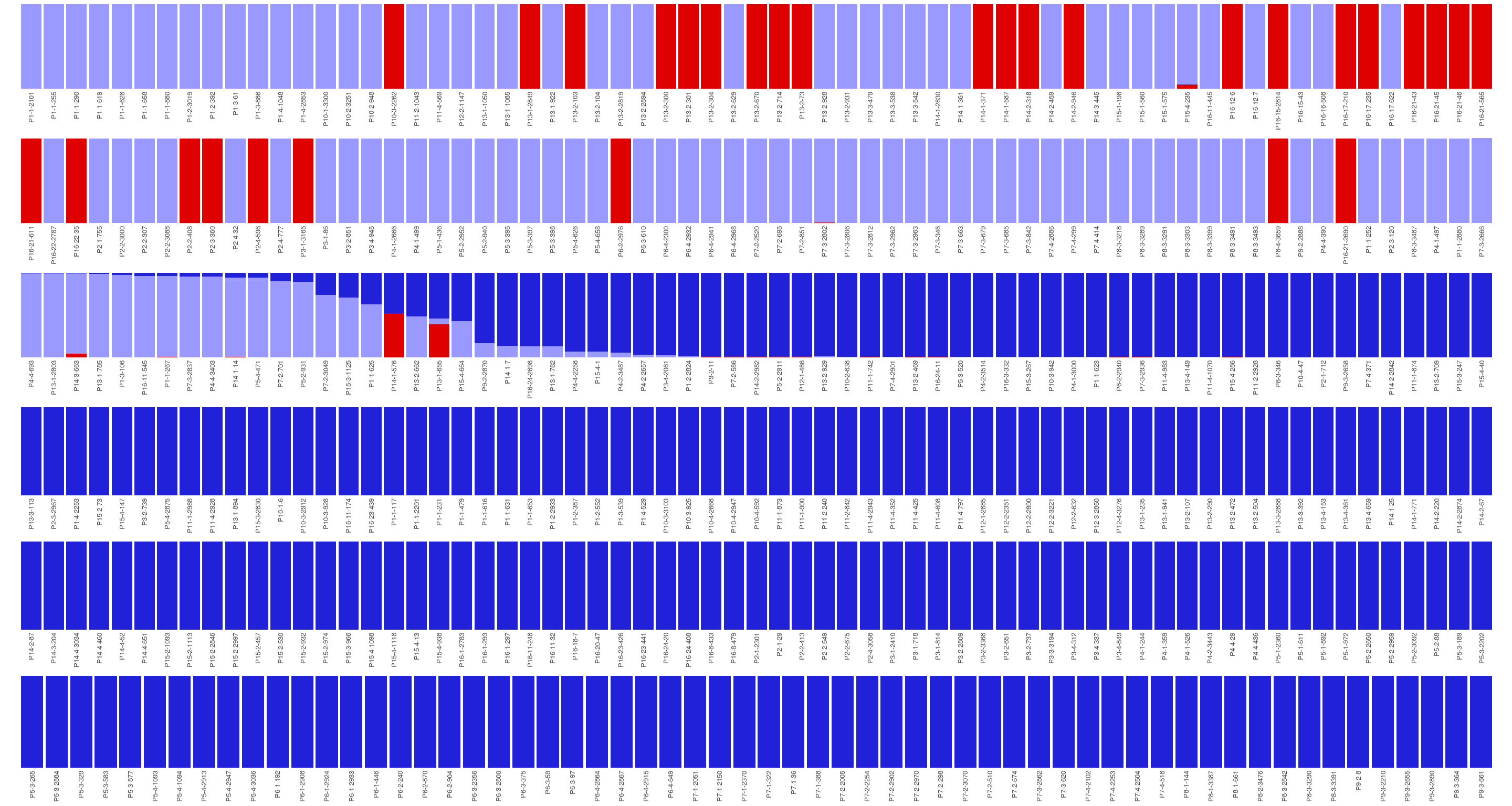
Figure 15.3: Population structure of Paracou individuals for K = 2. Dark blue is associated to S. globulifera morphotype; whereas light blue is associated to S. sp1
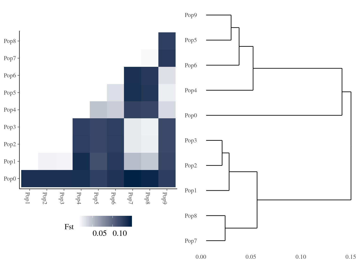
Figure 15.4: Clusters Fst relations for K=10.
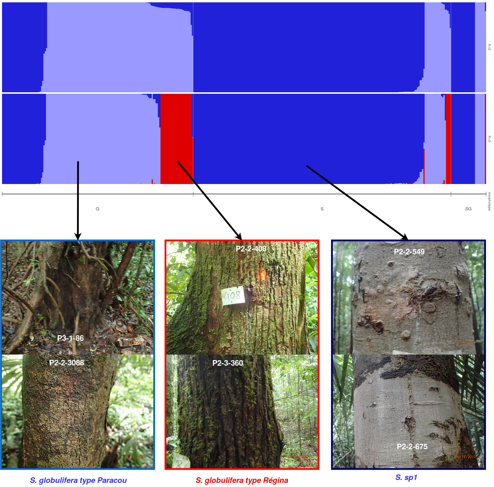
Figure 15.5: The Symphonia globulifera morphotypes identified in the field. The three morphottypes are identified with their bark with S. sp1 having a light grey thin and smooth bark, the S. globulifera type Paracou having a dark and intermediate thin and smooth bark compared to the thck and lashed bark of S. globulifera type Regina.
15.2 Spatial
Gene pools spatial distribution didn’t revealed much. Few individuals with a morphotype associated to the wrong ecotype have been reassigned with their gene pool the gene pool corresponding to the “good” ecotype (e.g. P13-4-361 previously presented as the S. globulifera morphotype living in plateau belong to the S. sp1 gene pool). But we still have individual with ecotypes not matching their gene pool, especially in subplot1 1 of plot 1 where there is a mix of gene pools in the bottomland but with a lot of hybridization ! In a nutshell, there are interessant patterns that deserve further detailed investigations (to be continued in association genomics).
Figure 15.6: Membership to the Symphonia globulifera gene pool for Paracou individuals.
15.3 Mismatch
Looking into detail for S. globulifera 2 commonly described morphotypes (Fig. 15.3), we have 32 individuals belonging to S. sp1 phenotype, 5 admixed individuals and finally 113 individuals with matching morhpotype and cluster (70%). Whereas for S. sp1 morphotype, we have 20 individuals belonging to S. globulifera phenotype, 7 admixed individuals and finally 180 individuals with matching morhpotype and cluster (88%). And last but not least, individuals identified as mixed morphotype on the field included 9 S. globulifera cluster and 19 S. sp1 cluster. Consequently including admixed indivduals we have 146 individuals in the S. globulifera cluster against 239 in the S. sp1 cluster.
We doubled checked (i) individuals with a mismatch between morphotype in Paracou data base (Pascal Petronelli identification) and gene pool attribution, (ii) Symphonia globulifera type Regina individuals, and (iii) admixed individuals with a blind-identification on the field. Most of them were failed first-identification and not an issue with gene pool attribution (Field result). Among 68 individuals, 59 were correct with blind-identification (87%) and 9 could be a possible error (13% of mismatch, 2% of the total number of sampled individuals).
Figure 15.7: Membership to the Symphonia globulifera gene pool for mismatch.
15.4 Environmental
Gene pools distribution along topographic wetness index and relative elevation is similar to morphotype distribution, revealing the two classical and clear morphotype-ecotype assocaitions of S. sp1 and S. globulifera. Nevertheless, we can noticed that S. globulifera type Régina grows in habitats even wetter than S. globulifera type Paracou as revealed by the topographic wetness index and not the relative elevation (so the position in the watershed matters). Gene pools association to the environment will be further explored with environmental genomics, to identify SNPs specifically associated to the topographic association.
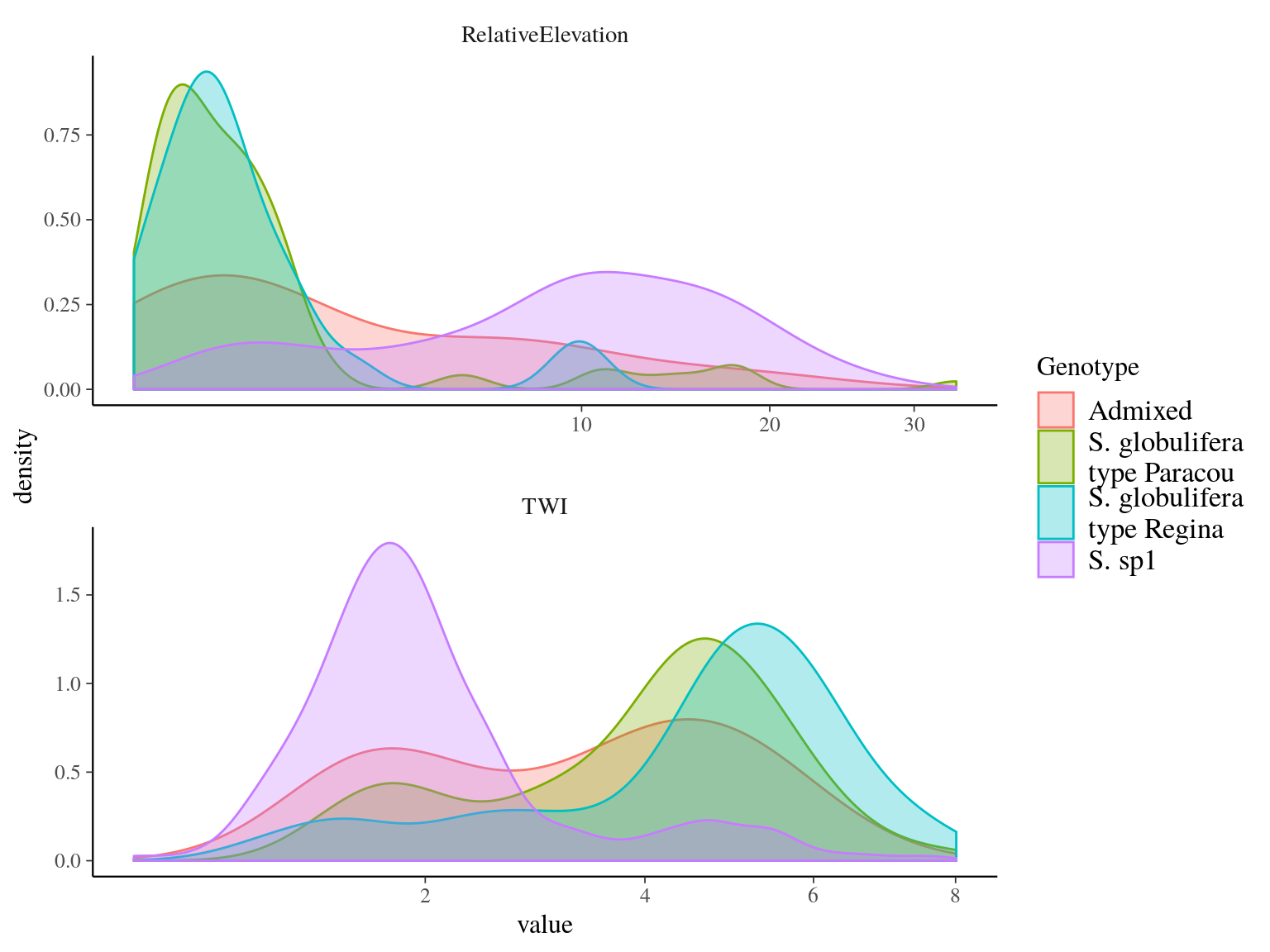
Figure 15.8: Gene pools distribution along topgraphic wetness index and relative elevation for Paracou individuals.
15.5 Kinship
We calculated kinship matrix (Fig. ??) for every individuals to be used in genomic scan to control for population structure. 19 individual, belonging to all gene pools, had only negative kinship values (Fig 15.11). After investigation it seems that these individuals are individuals without family in Paracou with null kinship with other individuals of their gene pools and negative values with other individuals of other gene pools. Interestingly though individuals with only null or negative kinship were all located on the limit of Paracou plots (Fig 15.12).
module load bioinfo/plink-v1.90b5.3
plink \
  --bfile symcapture.all.biallelic.snp.filtered.nonmissing.paracou \
  --allow-extra-chr \
  --recode vcf-iid \
  --out symcapture.all.biallelic.snp.filtered.nonmissing.paracou
vcftools --gzvcf  symcapture.all.biallelic.snp.filtered.nonmissing.paracou.vcf.gz  --relatedness2
# an estimated kinship coefficient range >0.354, [0.177, 0.354], [0.0884, 0.177] and [0.0442, 0.0884] corresponds to duplicate/MZ twin, 1st-degree, 2nd-degree, and 3rd-degree relationships respectively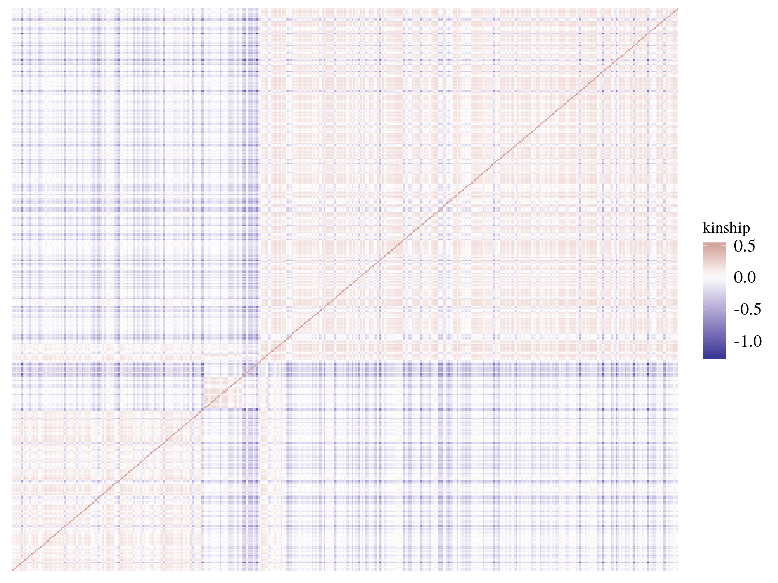
Figure 15.9: Individuals kinship matrix.
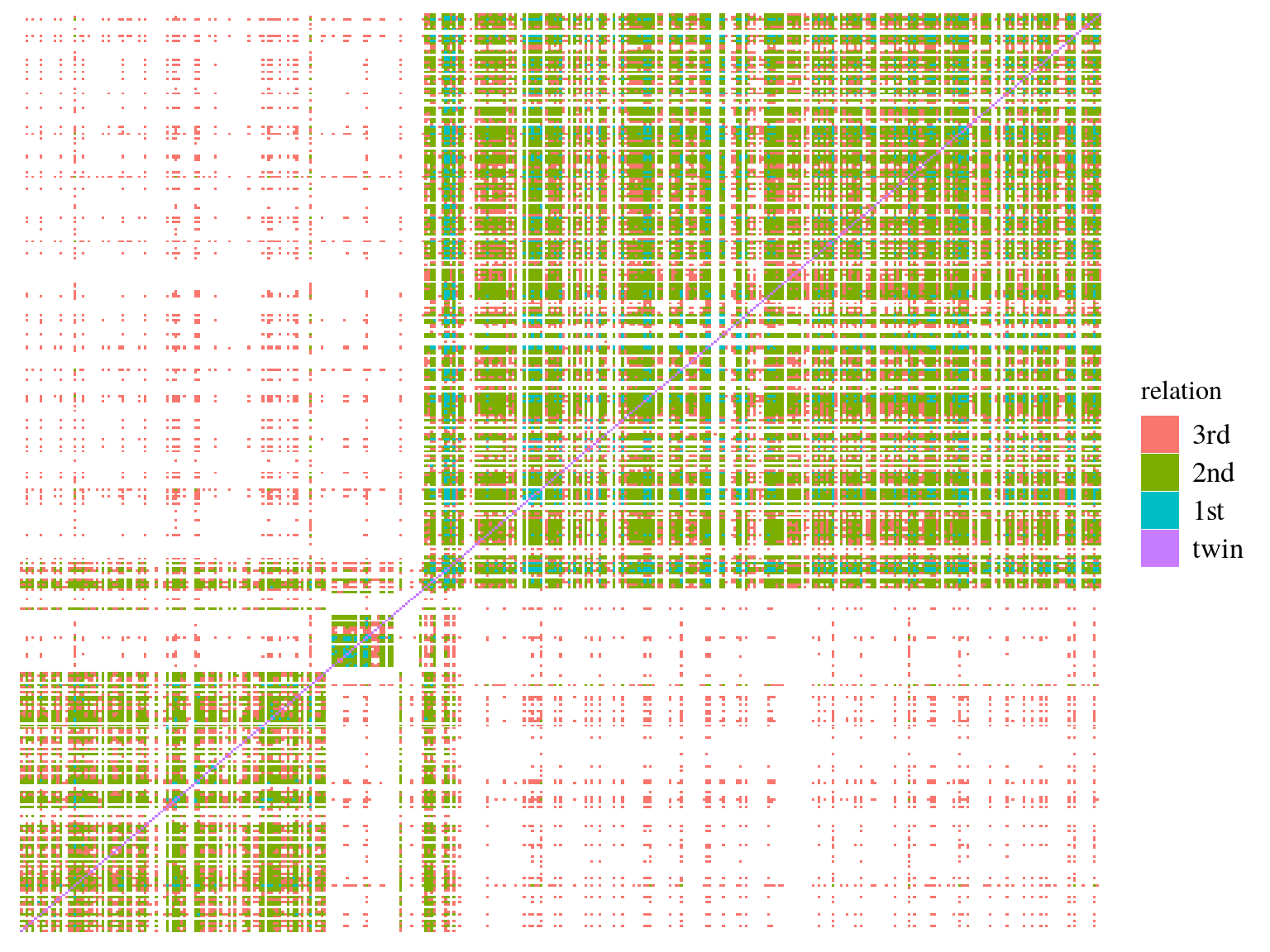
Figure 15.10: Individuals kinship matrix.
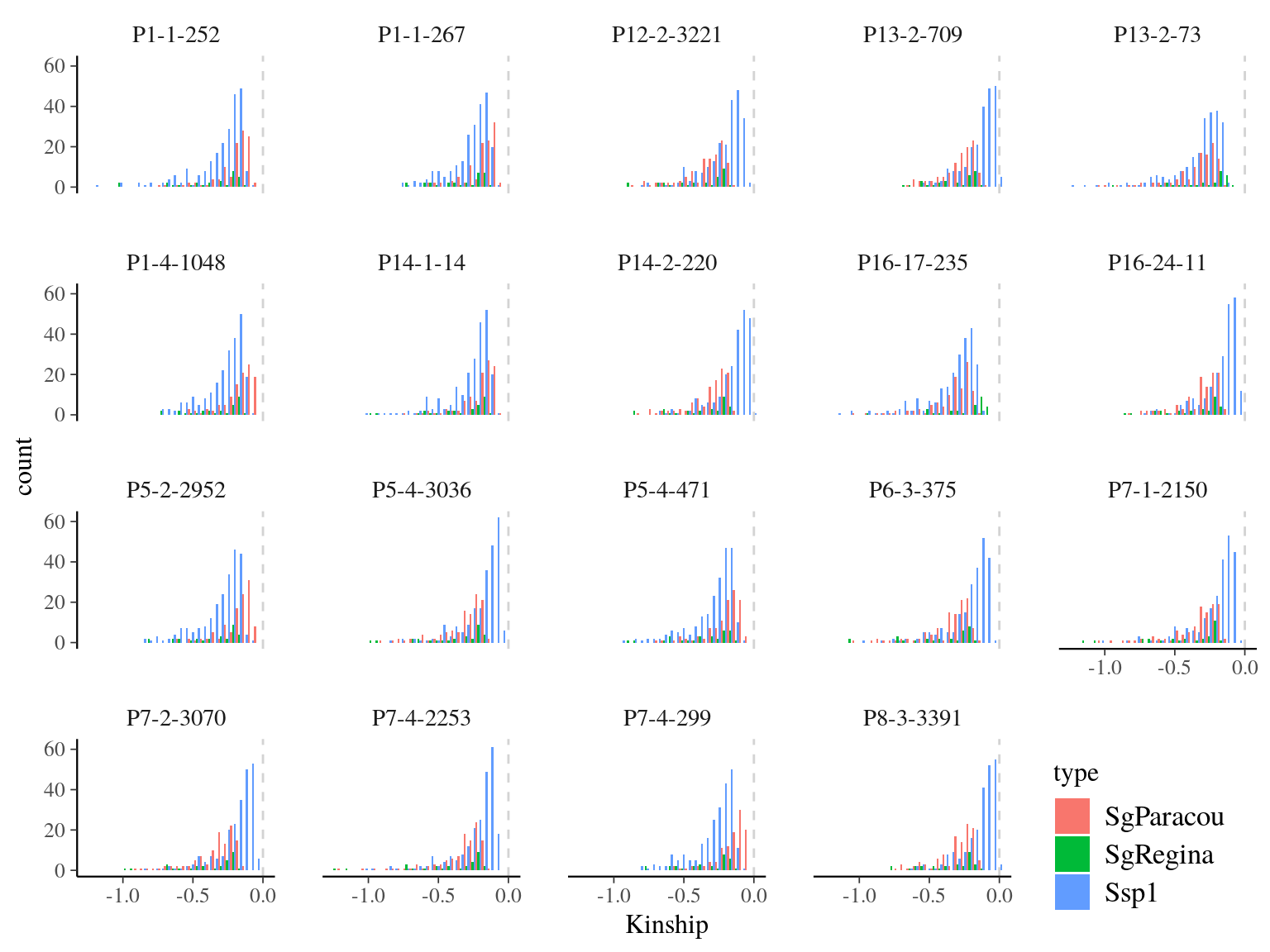
Figure 15.11: Kinship distribution for individuals with only null or negative kinship.
Figure 15.12: Map of individuals with only null or negative kinship.
15.6 Spatial auto-correlation
plink=~/Tools/plink_linux_x86_64_20190617/plink
$plink \
  --bfile ../paracou/symcapture.all.biallelic.snp.filtered.nonmissing.paracou \
  --allow-extra-chr \
  --keep sp1.fam \
  --recode vcf-iid \
  --thin-count 10000 \
  --out sp1
snps <- vroom::vroom(file.path(path, "..", "variantCalling", "spagedi", "sp1.genpop"), skip = 10002,
col_names = c("Lib", "Lat", "Long", paste0("SNP", 1:10000)))
XY <- mutate(snps, Ind = gsub(".g.vcf", "", Lib)) %>%
dplyr::select(Ind) %>%
left_join(dplyr::select(trees, Ind, Xutm, Yutm))
snps$Lat <- XY$Xutm
snps$Long <- XY$Yutm
write_tsv(snps, path = file.path(path, "..", "variantCalling", "spagedi", "sp1.spagedi.in"), col_names = T)// #ind #cat #coord #loci #dig/loc #ploidy// this an example (lines beginning by // are comment lines)
230 0 2 10000 3 2
6 10 25 50 100 150 200Locus intra-individual (inbreeding coef) 1 2 3 4 5 6 7 average 0-2704.88 b-lin(slope linear dist) b-log(slope log dist) ALL LOCI -0.0480 0.0079 0.0049 0.0046 0.0036 0.0035 0.0023 -0.0001 0.0001 -1.34448E-06 -0.00128963